Page 210 - Video Coding for Mobile Communications Efficiency, Complexity, and Resilience

Section 8.5. Simulation Results 187

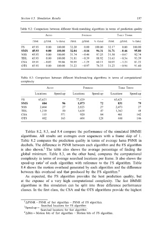
Table 8.2: Comparison between di+erent block-matching algorithms in terms of prediction quality
AKIYO FOREMAN TABLE TENNIS
PSNR 7PSNR % Global PSNR 7PSNR % Global PSNR 7PSNR % Global
FS 45.93 0.00 100.00 32.20 0.00 100.00 32.17 0.00 100.00
SMS 45.93 0.00 100.00 32.04 −0:16 94.31 31.71 −0:46 95.80
NSS 45.93 0.00 100.00 31.74 −0:46 87.25 31.50 −0:67 92.74
TDL 45.93 0.00 100.00 31.81 −0:39 88.92 31.63 −0:54 93.39
CSA 45.91 −0:02 99.86 30.95 −1:25 60.11 30.93 −1:24 81.23
OTS 45.93 0.00 100.00 31.23 −0:97 76.35 31.23 −0:94 91.60

Table 8.3: Comparison between di+erent blockmatching algorithms in terms of computational
complexity

AKIYO FOREMAN TABLE TENNIS
Locations Speed-up Locations Speed-up Locations Speed-up
FS 65,621 – 77,439 – 65,621 –
SMS 684 96 1,073 72 831 79
NSS 2,464 27 2,823 27 2,473 27
TDL 1,310 50 1,638 47 1,362 48
CSA 115 571 920 84 461 142
OTS 402 163 604 128 448 146

Tables 8.2, 8.3, and 8.4 compare the performance of the simulated BMME
algorithms. All results are averages over sequences with a frame skip of 1.
Table 8.2 compares the prediction quality in terms of average luma PSNR in
decibels. The di+erence in PSNR between each algorithm and the FS algorithm
2
is also shown. The table also shows the average percentage of :nding the
global minimum. Table 8.3, on the other hand, compares the computational
complexity in terms of average searched locations per frame. It also shows the
3
speed-up ratio of each algorithm with reference to the FS algorithm. Table
8.4 shows the motion overhead generated by each algorithm and the di+erence
between this overhead and that produced by the FS algorithm. 4
As expected, the FS algorithm provides the best prediction quality, but
at the expense of a very high computational complexity. The fast BMME
algorithms in this simulation can be split into three di+erence performance
classes. In the :rst class, the CSA and the OTS algorithms provide the highest

2 7PSNR = PSNR of fast algorithm − PSNR of FS algorithm.
Searched locations for FS algorithm
3 Speed-up = .
Searched locations for fast algorithm
4 7Bits = Motion bits of fast algorithm − Motion bits of FS algorithm.