Page 176 - Vogel's TEXTBOOK OF QUANTITATIVE CHEMICAL ANALYSIS

4 ERRORS AND STATlSTlCS

Total sum of squares = (0.0269 + 0.0157 + 0.0539) - C.F.
= 0.0965 - 0.0234 = 0.073 1
(d) The between-treatment (analyst) surn of squares. The sum of the squares of
each individual column is divided by the number of results in each column,
and then the correction factor is subtracted.
Between sum of squares = 6(0.292 + 0.21 + 0.452) - 0.0234
= 0.0593
(e) The within-sample surn of squares. The between sum of squares is subtracted
from the total sum of squares.
0.0731 - 0.0593 = 0.0138
(f) The degrees of freedom (v). These are obtained as follows:
The total number of degrees of freedom v = N - 1 = 11
The between-treatment degrees of freedom v = C - 1 = 2
The within-sample degrees of freedom v = (N - 1 ) - ( C - 1 ) = 9
where C is the number of columns (in this example, the number of analysts).
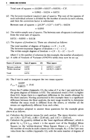
(g) A table of Analysis of Variance (ANOVA table) may now be set up.

Source of variation Sum of squares d.f. Mean square
'Between analysts' 0.0593 2 0.0593/2 = 0.0297
'Within titrations' 0.0138 9 0.0138/9 = 0.00153

Total 0.073 1 11

(h) The F-test is used to compare the two mean squares:

From the F-tables (Appendix 13), the value of F at the 1 per cent level for
the given degrees of freedom is 8.02. The calculated result (19.41) is higher
than 8.02; hence there is a significant difference in the results obtained by
the three analysts. Having ascertained in this example there is a significant
difference between the three analysts, the next stage would be to determine
whether the mean result is different from the others, or whether al1 the
means are significantly different from each other.
The procedure adopted to answer these questions for the example given
above is as follows:
(a) Calculate the titration means for each analyst. The mean titration values
are X (A) = 22.57 mL; X (B) = 22.45 mL; and X (C) = 22.61 mL.
(b) Calculate the quantity defined as the 'least significant difference', which is
-
given by s J2/n to.o, where s is the square root of the Residual Mean
Square, Le. the 'within-titration' Mean Square. Hence s = dm; is
n
the number of results in each column (in this example, 4); t is the 5 percent
value from the t-tables (Appendix 12), with the same number of degrees of