Page 73 - Water and Wastewater Engineering Design Principles and Practice

2-16 WATER AND WASTEWATER ENGINEERING

that it assumes that the sequence of events leading to a drought or flood will be the same in the
future as it was in the past. More sophisticated techniques have been developed to overcome this
disadvantage. These techniques are left for advanced hydrology classes.
The Rippl procedure for determining the storage volume is an application of the mass bal-
ance method of analyzing problems. In this case it is assumed that the only input is the flow into
the reservoir ( Q in ) and that the only output is the flow out of the reservoir ( Q out ). Therefore,with
the assumption that the density term cancels out because the change in density across the reser-
voir is negligible,
dS d()In d(Out )
(2-2)
dt dt dt
becomes

dS
Q out (2-3)
Q
in
dt
If both sides of the equation are multiplied by dt, the inflow and outflow become volumes (flow
rate time volume), that is,
dt
Q
Q )()
dS ( in dt ( out )() (2-4)
By substituting finite time increments ( t ), the change in storage is then

)
) (Qout
(Qin )( t )( t S (2-5)
By cumulatively summing the storage terms, the size of the reservoir can be estimated. For
water supply reservoir design, Q out is the demand, and zero or positive values of storage ( S )
indicate there is enough water to meet the demand. If the storage is negative, then the reservoir
must have a capacity equal to the absolute value of cumulative storage to meet the demand. This
is illustrated in the following example.

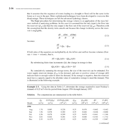
Example 2-3. Using the data in Table 2-7 , determine the storage required to meet Nosleep’s
3
demand of 0.25 m /s for the period from August 1994 through January 1997.
Solution. The computations are summarized in the table below.

Q in (0.05)(Q in ) (0.05)(Q in )( t) Q out Q out ( t) S S ( S)
3 3 6 3 3 6 3 6 3 6 3
Month (m /s) (m /s) (10 m ) (m /s) (10 m ) (10 m ) (10 m )
1994
Aug 1.70 0.085 0.228 0.25 0.670 0.442 0.442
Sep 1.56 0.078 0.202 0.25 0.648 0.446 0.888
Oct 1.56 0.078 0.209 0.25 0.670 0.461 1.348
Nov 2.04 0.102 0.264 0.25 0.648 0.384 1.732
Dec 2.35 0.1175 0.315 0.25 0.670 0.355 2.087
(continued)