Page 434 - Water and wastewater engineering

GRANULAR FILTRATION 11-7

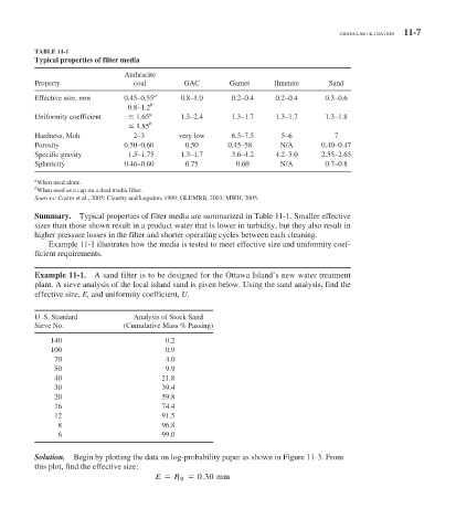
TABLE 11-1
Typical properties of filter media
Anthracite
Property coal GAC Garnet Ilmenite Sand

Effective size, mm 0.45–0.55 a 0.8–1.0 0.2–0.4 0.2–0.4 0.3–0.6
0.8–1.2 b
Uniformity coefficient 1.65 a 1.3–2.4 1.3–1.7 1.3–1.7 1.3–1.8
1.85 b
Hardness, Moh 2–3 very low 6.5–7.5 5–6 7
Porosity 0.50–0.60 0.50 0.45–58 N/A 0.40–0.47
Specific gravity 1.5–1.75 1.3–1.7 3.6–4.2 4.2–5.0 2.55–2.65
Sphericity 0.46–0.60 0.75 0.60 N/A 0.7–0.8

a
When used alone.
b
When used as a cap on a dual media filter.
Sources: Castro et al., 2005; Cleasby and Logsdon, 1999; GLUMRB, 2003; MWH, 2005.
Summary. Typical properties of filter media are summarized in Table 11-1 . Smaller effective
sizes than those shown result in a product water that is lower in turbidity, but they also result in
higher pressure losses in the filter and shorter operating cycles between each cleaning.
Example 11-1 illustrates how the media is tested to meet effective size and uniformity coef-
ficient requirements.

Example 11-1. A sand filter is to be designed for the Ottawa Island’s new water treatment
plant. A sieve analysis of the local island sand is given below. Using the sand analysis, find the
effective size, E, and uniformity coefficient, U.

U. S. Standard Analysis of Stock Sand
Sieve No. (Cumulative Mass % Passing)
140 0.2
100 0.9
70 4.0
50 9.9
40 21.8
30 39.4
20 59.8
16 74.4
12 91.5
8 96.8
6 99.0

Solution. Begin by plotting the data on log-probability paper as shown in Figure 11-3 . From
this plot, find the effective size:
E 0 30. mm
P 10