Page 266 - Well Logging and Formation Evaluation

256 Well Logging and Formation Evaluation

trum would correspond to the frequency content of the music. Taking out
some components in the frequency spectrum is analagous to using a
graphic equalizer on a household stereo. Filtering usually refers to ma-
nipulating the amplitude or phase spectra to take out unwanted compo-
nents. Since the transform process is reversible, a new “log” may be
constructed from the filtered components.

A4.3 NORMAL (GAUSSIAN) DISTRIBUTIONS

The normal probability curve is defined by:

2
- (
-
px) = [exp 05 ( * x m) s 2 )] ( ( *2 p ) *s ) (A4.1)
(
.
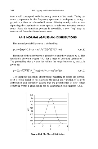
The mean of the distribution is given by m and the variance by s. This
function is shown in Figure A4.3, for a mean of zero and variance of 1.
The probability that a value lies within the range between x 1 and x 2 is
given by:
x 2 2 2
-
.
p = (2 (2* p ) )* Ú exp - ( 0 5* ( x m) s ) dx (A4.2)
x 1
It so happens that many distributions occurring in nature are normal,
so it is often useful to just calculate the mean and variation of a given
distribution and thereafter assume that the probabilities of new values
occurring within a given range can be calculated using equation A4.2.

0.45
0.4
0.35
0.3
p(x) 0.25
0.2
0.15
0.1
0.05
0
–4 –2 0 2 4
x

Figure A4.3 The Normal Distribution