Page 167 - Wind Energy Handbook

UNSTEADY FLOW – DYNAMIC INFLOW 141

400

Measurement
2D coefficients
300 3D coefficients
Aerodynamic power (kW) 200

100

0
0 10 20 30
Wind speed (m/s)

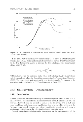
Figure 3.75 A Comparison of Measured and Snel’s Predicted Power Curves for a NOR-
TANK 300 kW Turbine

If the linear part of the static, two-dimensional, C l Æ curve is extended beyond
the stall then let ˜C l be the difference between the two curves. Then the correction
to the two-dimensional curve to account for the rotational, three-dimensional,
2
effects is 3(c=r) ˜C l .
2
c
þ 3 (3:190)
C l 3-D ¼ C l 2-D ˜C l
r
) lift coefficients
Table 3.2 compares the measured static (C l 2-D ) and rotating (C l 3-D
with the calculated values for the rotating values using Snel’s correction of Equation
(3.190). The correction is quite good and is very simple to apply. An example of the
correction is given by Snel et al. (1993) and is shown in Figure 3.75.

3.13 Unsteady flow – Dynamic inflow

3.13.1 Introduction

Natural winds are almost never steady in either strength or direction and so it is
seldom that the conditions for the momentum theory apply. It takes a finite time for
the wind to travel from far upwind of a rotor to far downwind and in that time
wind conditions will change so an equilibrium state is never achieved. Even if the
‘average’ wind speed changes only slowly small-scale turbulence will cause a
continuous unsteadiness in the velocities impinging on a rotor blade.
Several approximate solutions offer themselves for the determination of the