Page 167 - Characterization and Properties of Petroleum Fractions - M.R. Riazi

P2: IML/FFX
P1: IML/FFX
AT029-Manual
AT029-Manual-v7.cls
June 22, 2007
AT029-03
3. CHARACTERIZATION OF PETROLEUM FRACTIONS 147
5
90
10
70
80
95
40
50
Vol%
60
20
30
330
ASTM, F IBP QC: IML/FFX 350 T1: IML 366 380 14:23 390 404 417 433 450 469 482 FBP
500
342
◦
TBP, F 258 295 312 337 358 . . . 402 . . . 442 . . . 486 499 . . .
◦
SG . . . 0.772 0.778 0.787 0.795 . . . 0.817 . . . 0.824 . . . 0.829 0.830 . . .
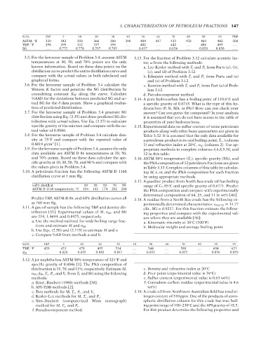
3.5. For the kerosene sample of Problem 3.4, assume ASTM 3.13. For the fraction of Problem 3.12 calculate acentric fac-
temperatures at 30, 50, and 70% points are the only tor, ω from the following methods:
known information. Based on these data points on the a. Lee–Kesler method with T c and P c from Parts (a), (b),
distillation curve predict the entire distillation curve and (c), and (d) of Problem 3.12.
compare with the actual values in both tabulated and b. Edmister method with T c and P c from Parts and (a)
graphical forms. and (e) of Problem 3.12.
3.6. For the kerosene sample of Problem 3.4 calculate the c. Korsten method with T c and P c from Part (a) of Prob-
Watson K factor and generate the SG distribution by lem 3.12.
considering constant K W along the curve. Calculate d. Pseudocomponent method
%AAD for the deviations between predicted SG and ac- 3.14. A pure hydrocarbon has a boiling point of 110.6 C and
◦
tual SG for the 8 data points. Show a graphical evalua- a specific gravity of 0.8718. What is the type of this hy-
tion of predicted distribution. drocarbon (P, N, MA, or PA)? How can you check your
3.7. For the kerosene sample of Problem 3.4 generate SG answer? Can you guess the compound? In your analysis
distribution using Eq. (3.35) and draw predicted SG dis- it is assumed that you do not have access to the table of
tribution with actual values. Use Eq. (3.37) to calculate properties of pure hydrocarbons.
specific gravity of the mixture and compare with the ac- 3.15. Experimental data on sulfur content of some petroleum
tual value of 0.8086. products along with other basic parameters are given in
3.8. For the kerosene sample of Problem 3.4 calculate den- Table 3.32. It is assumed that the only data available for
sity at 75 F and compare with the reported value of a petroleum product is its mid boiling point, T b , (column
◦
3
0.8019 g/cm [1]. 1) and refractive index at 20 C, n 20 (column 2). Use ap-
◦
3.9. For the kerosene sample of Problem 3.4, assume the only propriate methods to complete columns 4,6,8,9,10, and
data available are ASTM D 86 temperatures at 30, 50, 12 in this table.
and 70% points. Based on these data calculate the spe- 3.16. ASTM 50% temperature (T b ), specific gravity (SG), and
cific gravity at 10, 30, 50, 70, and 90 % and compare with the PNA composition of 12 petroleum fractions are given
the values given in Problem 3.4. in Table 3.33. Complete columns of this table by calculat-
3.10. A petroleum fraction has the following ASTM D 1160 ing M, n, m, and the PNA composition for each fraction
distillation curve at 1 mm Hg: by using appropriate methods.
3.17. A gasoline product from North Sea crude oil has boiling
vol% distilled 10 30 50 70 90 range of C 5 -85 C and specific gravity of 0.6771. Predict
◦
ASTM D 1160 temperature, C 104 143 174 202 244 the PNA composition and compare with experimentally
◦
determined composition of 64, 25, and 11 in wt% [46].
Predict TBP, ASTM D 86, and EFV distillation curves all 3.18. A residue from a North Sea crude has the following ex-
at 760 mm Hg. perimentally determined characteristics: ν 99(210) = 14.77
3.11. A gas oil sample has the following TBP and density dis- cSt., SG = 0.9217. For this fraction estimate the follow-
tribution [32]. Experimental values of M, n 20 , and SG ing properties and compare with the experimental val-
are 214, 1.4694, and 0.8475, respectively. ues where they are available [46]:
a. Use the method outlined for wide boiling range frac- a. Kinematic viscosity at 38 C (100 F)
◦
◦
tions and estimate M and n 20 . b. Molecular weight and average boiling point
b. Use Eqs. (2.50) and (2.115) to estimate M and n
c. Compare %AD from methods a and b.
Vol% IBP 5 10 20 30 40 50 60 70 80 90 95
TBP, F 420 451 470 495 514 . . . 544 . . . 580 . . . 604 621
◦
d 20 . . . 0.828 0.835 0.843 0.847 . . . 0.851 . . . 0.855 . . . 0.856 0.859
3.12. A jet naphtha has ASTM 50% temperature of 321 F and
◦
specific gravity of 0.8046 [1]. The PNA composition of
this fraction is 19, 70, and 11%, respectively. Estimate M, c. Density and refractive index at 20 C
◦
n 20 , d 20 , T c , P c , and V c from T b and SG using the following d. Pour point (experimental value is 39 C)
◦
methods: e. Sulfur content (experimental value is 0.63 wt%)
a. Riazi–Daubert (1980) methods [38]. f. Conradson carbon residue (experimental value is 4.6
b. API-TDB methods [2]. wt%)
c. Twu methods for M, T c , P c , and V c . 3.19. A crude oil from Northwest Australian field has total ni-
d. Kesler–Lee methods for M, T c , and P c . trogen content of 310 ppm. One of the products of atmo-
e. Sim–Daubert (computerized Winn nomograph) spheric distillation column for this crude has true boil-
method for M, T c , and P c . ing point range of 190–230 C and the API gravity of 45.5.
◦
f. Pseudocomponent method. For this product determine the following properties and

Copyright ASTM International
Provided by IHS Markit under license with ASTM Licensee=International Dealers Demo/2222333001, User=Anggiansah, Erick
No reproduction or networking permitted without license from IHS Not for Resale, 08/26/2021 21:56:35 MDT

--`,```,`,``````,`,````,```,,-`-`,,`,,`,`,,`---