Page 258 - Characterization and Properties of Petroleum Fractions - M.R. Riazi

T1: IML
P2: KVU/KXT
P1: KVU/KXT
QC: —/—
AT029-Manual-v7.cls
AT029-06
AT029-Manual
20:46
238 CHARACTERIZATION AND PROPERTIES OF PETROLEUM FRACTIONS
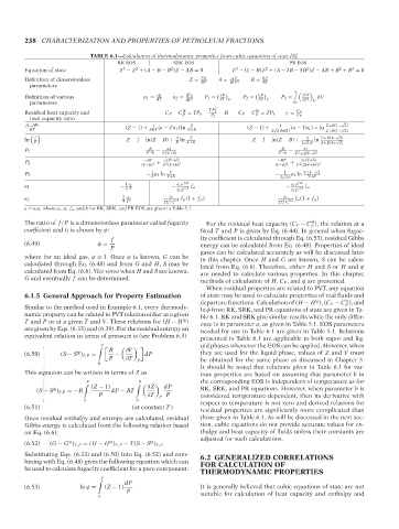
TABLE 6.1—Calculation of thermodynamic properties from cubic equations of state [8].
RK EOS June 22, 2007 SRK EOS PR EOS
2
2
2
3
3
2
3
2
Equation of state Z − Z + (A − B − B )Z − AB = 0 Z − (1 − B)Z + (A − 2B − 3B )Z − AB + B + B = 0
aP
Definition of dimensionless Z = PV A = R 2 T 2 B = bP
RT
RT
parameters
2
2
da
Definition of various a 1 = dT a 2 = d a P 1 = ∂ P P 2 = ∂ P P 3 = V
∂ P dV
∂T 2
∂T V
∂V T
dT 2
parameters ∞ V
ig TP 2 ig
Residual heat capacity and C P − C P = TP 3 − 1 − R C V − C V = TP 3 γ = C P
heat capacity ratio P 2 C V
√
H−H ig 1 (a − Ta 1 )ln Z 1 (a − Ta 1 ) × ln Z+B(1− 2)
√
√
RT (Z − 1) + bRT Z+B (Z − 1) + 2 2(bRT) Z+B(1+ 2)
√

A Z A Z+B(1− 2)
f
ln ln ln
√
√
P Z − 1 − ln(Z − B) + B Z+B Z − 1 − ln(Z − B) + 2 2 B Z+B(1+ 2)
R a 1 R a 1
P 1 − −
V−b V(V+b) V−b V 2 +2bV−b 2
−RT a(2V+b) −RT 2a(V+b)
P 2 + +
(V−b) 2 V 2 (V+b) 2 (V−b) 2 V 2 (2bV+b 2 ) 2
√
V
V+b− 2
1
1
P 3 − a 2 ln − √ a 2 ln
b V+b 2 2 b V+b
1 a a c α 1/2 a c α 1/2
a 1 − − f ω − f ω
2 T 1/2 1/2
T c T r T c T r
3 a a c a c
a 2 f ω (1 + f ω ) f ω (1 + f ω )
4 T 2 2 3/2 2 3/2
2T c T r 2T c T r
a = a c α, where a c , α, f ω ,and b for RK, SRK, and PR EOS are given in Table 5.1.
ig
The ratio of f/P is a dimensionless parameter called fugacity For the residual heat capacity (C P − C ), the relation at a
P
coefficient and it is shown by φ: fixed T and P is given by Eq. (6.44). In general when fugac-
f ity coefficient is calculated through Eq. (6.53), residual Gibbs
(6.49) φ = energy can be calculated from Eq. (6.48). Properties of ideal
P
gases can be calculated accurately as will be discussed later
where for an ideal gas, φ = 1. Once φ is known, G can be in this chapter. Once H and G are known, S can be calcu-
calculated through Eq. (6.48) and from G and H, S may be lated from Eq. (6.6). Therefore, either H and S or H and φ
calculated from Eq. (6.6). Vice versa when H and Sare known, are needed to calculate various properties. In this chapter,
G and eventually f can be determined.
methods of calculation of H, C P , and φ are presented.
When residual properties are related to PVT, any equation
6.1.5 General Approach for Property Estimation of state may be used to calculate properties of real fluids and
ig
ig
departure functions. Calculation of (H − H ), (C P − C ), and
P
Similar to the method used in Example 6.1, every thermody- ln φ from RK, SRK, and PR equations of state are given in Ta-
namic property can be related to PVT relation either at a given ble 6.1. RK and SRK give similar results while the only differ-
T and P or at a given T and V. These relations for (H − H ) ence is in parameter a, as given in Table 5.1. EOS parameters
ig
are given by Eqs. (6.33) and (6.39). For the residual entropy an needed for use in Table 6.1 are given in Table 5.1. Relations
equivalent relation in terms of pressure is (see Problem 6.3) presented in Table 6.1 are applicable to both vapor and liq-
uid phases whenever the EOS can be applied. However, when
R ∂V
P
ig
(6.50) (S − S ) T,P = − dP they are used for the liquid phase, values of Z and V must
P ∂T P be obtained for the same phase as discussed in Chapter 5.
0
It should be noted that relations given in Table 6.1 for var-
This equation can be written in terms of Z as ious properties are based on assuming that parameter b in
the corresponding EOS is independent of temperature as for
(Z − 1) P ∂ Z dP
P
ig
(S − S ) T,P =−R dP − RT RK, SRK, and PR equations. However, when parameter b is
P ∂T P P considered temperature-dependent, then its derivative with
0 0 respect to temperature is not zero and derived relations for
--`,```,`,``````,`,````,```,,-`-`,,`,,`,`,,`---
(6.51) (at constant T )
residual properties are significantly more complicated than
Once residual enthalpy and entropy are calculated, residual those given in Table 6.1. As will be discussed in the next sec-
Gibbs energy is calculated from the following relation based tion, cubic equations do not provide accurate values for en-
on Eq. (6.6): thalpy and heat capacity of fluids unless their constants are
adjusted for such calculations.
ig
ig
ig
(6.52) (G − G ) T,P = (H − H ) T,P − T(S − S ) T,P
Substituting Eqs. (6.33) and (6.50) into Eq. (6.52) and com- 6.2 GENERALIZED CORRELATIONS
bining with Eq. (6.48) gives the following equation which can FOR CALCULATION OF
be used to calculate fugacity coefficient for a pure component:
THERMODYNAMIC PROPERTIES
dP
P
(6.53) ln φ = (Z − 1) It is generally believed that cubic equations of state are not
P
0 suitable for calculation of heat capacity and enthalpy and
Copyright ASTM International
Provided by IHS Markit under license with ASTM Licensee=International Dealers Demo/2222333001, User=Anggiansah, Erick
No reproduction or networking permitted without license from IHS Not for Resale, 08/26/2021 21:56:35 MDT