Page 120 - Introduction to Statistical Pattern Recognition

102 Introduction to Statistical Pattern Recognition

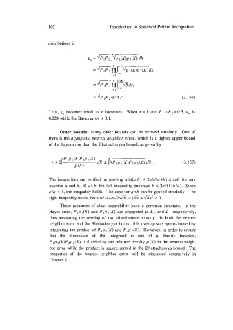
distributions is

= =hf;‘l3dxj
i=l
= G0.447” (3.156)
.

Thus, E,, becomes small as n increases. When n = 1 and P 1 =P 2 =OS, E, is
0.224 while the Bayes error is 0.1.

Other bounds: Many other bounds can be derived similarly. One of
them is the asymptotic nearesf neighbor error, which is a tighter upper bound
of the Bayes error than the Bhattacharyya bound, as given by

E I21 p1p1(x)p2p2(x) dX I IJP lpl(x)P2p2(x) dX . (3.157)
P (X)

The inequalities are verified by proving min[a,h] I 2ahl(a+b) 5 dab for any
positive a and h. If a>b, the left inequality becomes b < 2b/(l+b/a). Since
bla < 1, the inequality holds. The case for a<h can be proved similarly. The
right inequality holds, because a+h-2&6 = (& + dh)* 2 0.
These measures of class separability have a common structure. In the
Bayes error, P,p,(X) and P2p2(X) are integrated in L2 and L1 respectively,
thus measuring the overlap of two distributions exactly. In both the nearest
neighbor error and the Bhattacharyya bound, this overlap was approximated by
integrating the product of P pl(X) and P2p2(X). However, in order to ensure
that the dimension of the integrand is one of a density function,
P Ip (X)P2p2(X) is divided by the mixture density p(X) in the nearest neigh-
I
bor error while the product is square-rooted in the Bhattacharyya bound. The
properties of the nearest neighbor error will be discussed extensively in
Chapter 7.