Page 130 - Introduction to Statistical Pattern Recognition

112 Introduction to Statistical Pattern Recognition

(3.179)

where the inequalities are derived from In x I x - 1. The equalities in (3.178)
and (3.179) hold only when pl(X) = p2(X).
Thus, as m increases, E { s I o1 decreases and E { s I o2 increases in pro-
}
}
portion to m, while the standard deviations increase in proportion to &. This
is true regardless of p I (X) and p2(X) as long as p I (X) # p2(X). Therefore, the
density functions of s for o1 and o2 become more separable as m increases.
Also, by the central limit theorem, the density function of s tends toward a nor-
mal distribution for large m.

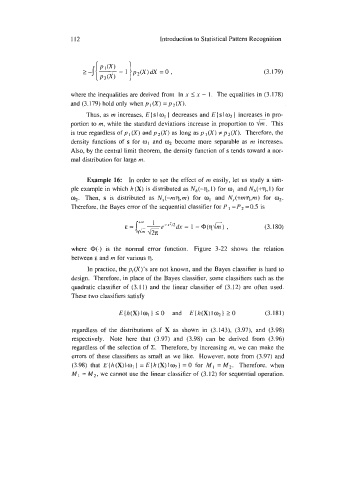
Example 16: In order to see the effect of m easily, let us study a sim-
ple example in which h (X) is distributed as Nh(-q, 1) for w, and Nh(+q, 1) for
02. Then, s is distributed as N,(-rnq,m) for o1 and N,(+mT,m) for 02.
Therefore, the Bayes error of the sequential classifier for P I = P2 = 0.5 is

(3.180)

where @(.) is the normal error function. Figure 3-22 shows the relation
between E and m for various q.
In practice, the pi(X)’s are not known, and the Bayes classifier is hard to
design. Therefore, in place of the Bayes classifier, some classifiers such as the
quadratic classifier of (3.1 1) and the linear classifier of (3.12) are often used.
These two classifiers satisfy

E(h(X)lwl} 10 and E{h(X)Io2} 20 (3.181)

regardless of the distributions of X as shown in (3.143), (3.97), and (3.98)
respectively. Note here that (3.97) and (3.98) can be derived from (3.96)
regardless of the selection of C. Therefore, by increasing m, we can make the
errors of these classifiers as small as we like. However, note from (3.97) and
(3.98) that E { h (X) o1 = E (h (X) 1 = 0 for MI Mz. Therefore, when
I
=
}
1%
=
MI M2, we cannot use the linear classifier of (3.12) for sequential operation.