Page 225 - Introduction to Statistical Pattern Recognition

5 Parameter Estimation 207

Section 3.3. First, we get the closed-form solution for the integration with
respect to X, and then take the one-dimensional integration with respect to o
numerically.
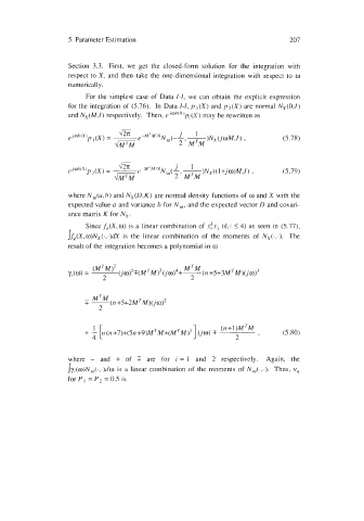
For the simplest case of Data 1-1, we can obtain the explicit expression
for the integration of (5.76). In Data 1-1, p , (X) and p2(X) are normal NX(O,I)
and NX(M,I) respectively. Then, e’oh(xip,(X) may be rewritten as

(5.78)

(5.79)

where N,(a,h) and NX(D,K) are normal density functions of w and X with the
expected value a and variance h for N,, and the expected vector D and covari-
ance matrix K for NX.
Since f,(X, o) is a linear combination of x;x, (k,L 5 4) as seen in (5.77),
is
Ifq(X,o)NX(.;)dX the linear combination of the moments of Nx(.,.). The
result of the integration becomes a polynomial in o

where - and + of T are for i = 1 and 2 respectively. Again, the
JY,(o)N,(.,.)do is a linear combination of the moments of N,(.,.). Thus, vy
for PI = P2 = 0.5 is