Page 226 - Introduction to Statistical Pattern Recognition

208 Introduction to Statistical Pattern Recognition

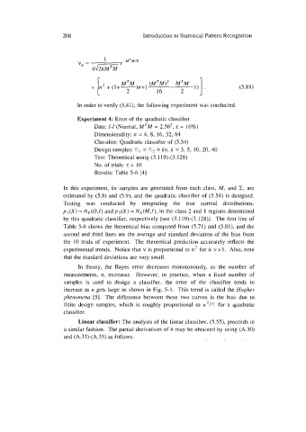
vq = 1 e -M 'MI8
4dsiiG

(LW'M)~ M'M I] (5.81)
---1
16 2

In order to verify (5.81), the following experiment was conducted.
Experiment 4: Error of the quadratic classifier
Data: I-I (Normal, MTM = 2.56*, E = 10%)
Dimensionality: n = 4, 8, 16, 32, 64
Classifier: Quadratic classifier of (5.54)
=
Design samples: ?I, kn, k = 3, 5, 10, 20, 40
=
?I2
Test: Theoretical using (3.119)-(3.128)
No. of trials: z = 10
Results: Table 5-6 [41
In this experiment, kn samples are generated from each class, Mi and Cj are
estimated by (5.8) and (5.9), and the quadratic classifier of (5.54) is designed.
Testing was conducted by integrating the true normal distributions,
p I(X) = Nx(O,I) and p2(X) = Nx(M,f), the class 2 and 1 regions determined
in
by this quadratic classifier, respectively [see (3.1 19)-(3.128)]. The first line of
Table 5-6 shows the theoretical bias computed from (5.71) and (5.81), and the
second and third lines are the average and standard deviation of the bias from
the 10 trials of experiment. The theoretical prediction accurately reflects the
experimental trends. Notice that v is proportional to n2 for n >> 1. Also, note
that the standard deviations are very small.
In theory, the Bayes error decreases monotonously, as the number of
measurements, n, increases. However, in practice, when a fixed number of
samples is used to design a classifier, the error of the classifier tends to
increase as n gets large as shown in Fig. 5-1. This trend is called the Hughes
phenomena [51. The difference between these two curves is the bias due to
finite design samples, which is roughly proportional to n2/n for a quadratic
classifier.
Linear classifier: The analysis of the linear classifier, (5.53, proceeds in
a similar fashion. The partial derivatives of h may be obtained by using (A.30)
and (A.33)-(A.35) as follows.