Page 362 - Introduction to Statistical Pattern Recognition

344 Introduction to Statistical Pattern Recognition

approaches a uniform (hyperelliptical) kernel, always with a smooth roll-off
(for finite m), and always with covariance r2Ai. Using this kernel allows us to
use kernel functions close to the uniform kernel, without having to worry about
the problem of equal density estimates.
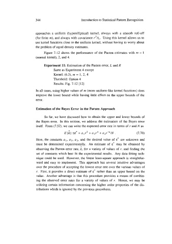
Figure 7-12 shows the performance of the Parzen estimates with m = 1
(normal kernel), 2, and 4.

Experiment 11: Estimation of the Parzen error, L and R
Same as Experiment 4 except
Kernel: (6.3), m = 1, 2, 4
Threshold: Option 4
Results: Fig. 7-12 [12]

In all cases, using higher values of rn (more uniform-like kernel functions) does
improve the lower bound while having little effect on the upper bounds of the
error.

Estimation of the Bayes Error in the Parzen Approach

So far, we have discussed how to obtain the upper and lower bounds of
the Bayes error. In this section, we address the estimation of the Bayes error
itself. From (7.52), we can write the expected error rate in terms of r and N as

(7.70)
Here, the constants ul, u2, a3, and the desired value of E* are unknown and
must be determined experimentally. An estimate of E* may be obtained by
A
observing the Parzen error rate, E, for a variety of values of r, and finding the
set of constants which best fit the experimental results. Any data fitting tech-
nique could be used. However, the linear least-square approach is straightfor-
ward and easy to implement. This approach has several intuitive advantages
over the procedure of accepting the lowest error rate over the various values of
r. First, it provides a direct estimate of E* rather than an upper bound on the
value. Another advantage is that this procedure provides a means of combin-
ing the observed error rates for a variety of values of r. Hence, we may be
utilizing certain information concerning the higher order properties of the dis-
tributions which is ignored by the previous procedures.