Page 276 - Petroleum Production Engineering, A Computer-Assisted Approach

Guo, Boyun / Computer Assited Petroleum Production Engg 0750682701_chap18 Final Proof page 276 4.1.2007 10:04pm Compositor Name: SJoearun

18/276 PRODUCTION ENHANCEMENT
2,000 using simultaneous solving approaches. Commercial soft-
ware to perform this type of computations include ReO,
GAP, HYSYS, FAST Piper, and others.
1,500
Operating Rate (stb/day) 1,200 Field-level production optimizations are carried out with
18.8.2 Optimization Approaches
two distinct approaches: (a) the simulation approach and
(b) the optimization approach.
800
18.8.2.1 Simulation Approach
The simulation approach is a kind of trial-and-error
400
approach. A computer program simulates flow conditions
(pressures and flow rates) with fixed values of variables in
each run. All parameter values are input manually before
0 each run. Different scenarios are investigated with differ-
0 1.5 3 4.5 6
ent sets of input data. Optimal solution to a given problem
Life Gas Injection Rate (MMscf/day) is selected on the basis of results of many simulation runs
with various parameter values. Thus, this approach is
Figure 18.12 A typical gas lift performance curve of a more time consuming.
high-productivity well.
18.8.2.2 Optimization Approach
18.8 Oil and Gas Production Fields The optimization approach is a kind of intelligence-based
approach. It allows some values of parameters to be
An oil or gas field integrates wells, flowlines, separation
facilities, pump stations, compressor stations, and trans- determined by the computer program in one run. The
portation pipelines as a whole system. Single-phase and parameter values are optimized to ensure the objective
multiphase flow may exist in different portions in the function is either maximized (production rate as the
system. Depending on system complexity and the objective objective function) or minimized (cost as the objective
of optimization task, field level production optimization function) under given technical or economical constraints.
can be performed using different approaches. Apparently, the optimization approach is more efficient
than the simulation approach.
18.8.1 Types of Flow Networks 18.8.3 Procedure for Production Optimization
Field-level production optimization deals with complex The following procedure may be followed in production
flow systems of two types: (1) hierarchical networks and optimization:
(2) nonhierarchical networks. A hierarchical network is
defined as a treelike converging system with multiple in- 1. Define the main objective of the optimization study.
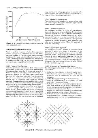
flow points (sources) and one outlet (sink). Figure 18.13 The objectives can be maximizing the total oil/gas
illustrates two hierarchical networks. Flow directions in production rate or minimizing the total cost of
this type of network are known. Fluid flow in this type of operation.
network can be simulated using sequential solving 2. Define the scope (boundary) of the flow network.
approach. Commercial software to perform this type of 3. Based on the characteristics of the network and fluid
computation are those system analysis (Nodal analysis) type, select a computer program.
programs such as FieldFlo and PipeSim, among others. 4. Gather the values of component/equipment param-
A nonhierarchical network is defined as a general eters in the network such as well-inflow performance,
system with multiple inflow points (sources) and multiple tubing sizes, choke sizes, flowline sizes, pump capacity,
outlets (sinks). Loops may exist, so the flow directions in compressor horsepower, and others.
some portions of the network are not certain. Figure 18.14 5. Gather fluid information including fluid compositions
presents a nonhierarchical network. Arrows in this figure and properties at various points in the network.
represent flow directions determined by a computer pro- 6. Gather the fluid-flow information that reflects the cur-
gram. Fluid flow in this type of network can be simulated rent operating point, including pressures, flow rates,
and temperatures at all the points with measurements.

Figure 18.13 Schematics of two hierarchical networks.