
Page 275 - Petroleum Production Engineering, A Computer-Assisted Approach
P. 275
Guo, Boyun / Computer Assited Petroleum Production Engg 0750682701_chap18 Final Proof page 275 4.1.2007 10:04pm Compositor Name: SJoearun
PRODUCTION OPTIMIZATION 18/275
200
RD = 0.4
180
RD = 0.6
160 RD = 0.8
Increase in Flow Rate (%) 120 RD = 1.4
RD = 1.0
140
RD = 1.2
RD = 1.6
RD = 1.8
100
RD = 2.0
80
60
40
20
0
0 10 20 30 40 50 60 70 80 90 100
Looped Line (%)
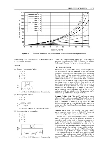
Figure 18.11 Effects of looped line and pipe diameter ratio on the increase of gas flow rate.
transmission; and (c) loop 3 miles of the 4-in. pipeline with Similar problems can also be solved using the spreadsheet
a 6-in. pipeline segment. program LoopedLines.xls. Table 18.2 shows the solution
to Example Problem 18.3 given by the spreadsheet.
Solution
18.7 Gas-Lift Facility
(a) Replace a portion of pipeline: Optimization of gas lift at the facility level mainly focuses
L ¼ 10 mi on determination of the optimum lift-gas distribution
L 1 ¼ 7mi among the gas-lifted wells. If lift-gas volume is not limited
L 2 ¼ 3mi by the capacity of the compression station, every well
D 1 ¼ 4in: should get the lift-gas injection rate being equal to its
D 2 ¼ 6in: optimal gas injection rate (see Section 18.3). If limited
lift-gas volume is available from the compression station,
v ffiffiffiffiffiffiffiffiffiffiffiffiffiffiffiffiffiffiffiffiffiffiffiffiffiffiffiffiffiffiffiffi
u the lift gas should be assigned first to those wells that will
u 10
u produce more incrementals of oil production for a given
q t u 4 16=3
¼ u incremental of lift-gas injection rate. This can be done by
q 1 t 7 þ 3 calculating and comparing the slopes of the gas-lift
4 16=3 6 16=3 performance curves of individual wells at the points of
adding more lift-gas injection rate. This principle can be
¼ 1:1668, or 16:68% increase in flow capacity:
illustrated by the following example problem.
(b) Place a parallel pipeline:
Example Problem 18.4 The gas-lift performance curves
D 1 ¼ 4in: of two oil wells are known based on Nodal analyses at well
D 2 ¼ 6in: level. The performance curve of Well A is presented in
p ffiffiffiffiffiffiffiffiffiffi p ffiffiffiffiffiffiffiffiffiffi Fig. 18.3 and that of Well B is in Fig. 18.12. If a total
q t 4 16=3 þ 6 16=3 lift-gas injection rate of 1.2 to 6.0 MMscf/day is available
¼ p ffiffiffiffiffiffiffiffiffiffi to the two wells, what lift-gas flow rates should be assigned
q 1 4 16=3
to each well?
¼ 3:9483, or 294:83% increase in flow capacity:
Solution Data used for plotting the two gas-lift
(c) Loop a portion of the pipeline:
performance curves are shown in Table 18.3. Numerical
L ¼ 10 mi derivatives (slope of the curves) are also included.
L 1 ¼ 7mi At each level of given total gas injection rate, the incre-
L 2 ¼ 3mi mental gas injection rate (0.6 MMscf/day) is assigned to
D 1 ¼ 4in: one of the wells on the basis of their performance curve
D 2 ¼ 6in:
slope at the present gas injection rate of the well. The
v ffiffiffiffiffiffiffiffiffiffiffiffiffiffiffiffiffiffiffiffiffiffiffiffiffiffiffiffiffiffiffiffiffiffiffiffiffiffiffiffiffiffiffiffiffiffiffiffiffiffiffiffiffiffiffiffiffiffiffiffiffiffiffiffi procedure and results are summarized in Table 18.4. The
u
u 10 results indicate that the share of total gas injection rate by
u
q t u 4 16=3 wells depends on the total gas rate availability and per-
¼ u 0 1 formance of individual wells. If only 2.4 MMscf/day of gas
u
q 3 u
u B L 1 L 3 C is available, no gas should be assigned to Well A. If only
t @ p ffiffiffiffiffiffiffiffiffiffi p ffiffiffiffiffiffiffiffiffiffi 2 þ 16=3 A 3.6 MMscf/day of gas is available, Well A should share
4 16=3 þ 6 16=3 4 one-third of the total gas rate. If only 6.0 MMscf/day of
gas is available, each well should share 50% of the total gas
¼ 1:1791, or 17:91% increase in flow capacity:
rate.