Page 274 - Petroleum Production Engineering, A Computer-Assisted Approach

Guo, Boyun / Computer Assited Petroleum Production Engg 0750682701_chap18 Final Proof page 274 4.1.2007 10:04pm Compositor Name: SJoearun

18/274 PRODUCTION ENHANCEMENT
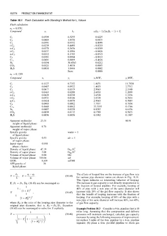
Table 18.1 Flash Calculation with Standing’s Method for k i Values
Flash calculation
n v ¼ 0:8791
Compound z i k i z i (k i 1)=[n v (k i 1) þ 1]
C 1 0.6599 6.5255 0.6225
C 2 0.0869 1.8938 0.0435
C 3 0.0591 0.8552 0:0098
i-C 4 0.0239 0.4495 0:0255
n-C 4 0.0278 0.3656 0:0399
i-C 5 0.0157 0.1986 0:0426
n-C 5 0.0112 0.1703 0:0343
C 6 0.0181 0.0904 0:0822
C 7þ 0.0601 0.0089 0:4626
N 2 0.0194 30.4563 0.0212
CO 2 0.0121 3.4070 0.0093
H 2 S 0.0058 1.0446 0.0002
Sum: 0.0000
n L ¼ 0.1209
Compound x i y i x i MW i y i MW i

C 1 0.1127 0.7352 1.8071 11.7920
C 2 0.0487 0.0922 1.4633 2.7712
C 3 0.0677 0.0579 2.9865 2.5540
i-C 4 0.0463 0.0208 2.6918 1.2099
n-C 4 0.0629 0.0230 3.6530 1.3356
i-C 5 0.0531 0.0106 3.8330 0.7614
n-C 5 0.0414 0.0070 2.9863 0.5085
C 6 0.0903 0.0082 7.7857 0.7036
C 7þ 0.4668 0.0042 53.3193 0.4766
N 2 0.0007 0.0220 0.0202 0.6156
CO 2 0.0039 0.0132 0.1709 0.5823
H 2 S 0.0056 0.0058 0.1902 0.1987
Apparent molecular 23.51 80.91
weight of liquid phase:
Apparent molecular 0.76
weight of vapor phase:
Specific gravity water ¼ 1
of liquid phase:
Specific gravity 0.81 air ¼ 1
of vapor phase:
Input vapor 0.958
phase z factor:
Density of liquid phase: 47.19 lb m =ft 3
Density of vapor phase: 2.08 lb m =ft 3
Volume of liquid phase: 0.04 bbl
Volume of vapor phase: 319.66 scf
GOR: 8,659 scf/bbl
API gravity of 56
liquid phase:

L 1 q t q 3 The effects of looped line on the increase of gas flow rate
Y ¼ , X ¼ : (18:44)
L q 3 for various pipe diameter ratios are shown in Fig. 18.11.
This figure indicates an interesting behavior of looping:
If, D 1 ¼ D 3 , Eq. (18.43) can be rearranged as The increase in gas capacity is not directly proportional to
the fraction of looped pipeline. For example, looping of
1
1 40% of pipe with a new pipe of the same diameter will
ð 1 þ XÞ 2
Y ¼ , (18:45) increase only 20% of the gas flow capacity. It also shows
1 that the benefit of looping increases with the fraction of
1
1 þ R 2:31 2 looping. For example, looping of 80% of the pipe with a
D
new pipe of the same diameter will increase 60%, not 40%,
where R D is the ratio of the looping pipe diameter to the of gas flow capacity.
original pipe diameter, that is, R D ¼ D 2 =D 3 . Equation
(18.45) can be rearranged to solve for X explicitly Example Problem 18.3 Consider a 4-in. pipeline that is 10
miles long. Assuming that the compression and delivery
1
X ¼ v ffiffiffiffiffiffiffiffiffiffiffiffiffiffiffiffiffiffiffiffiffiffiffiffiffiffiffiffiffiffiffiffiffiffiffiffiffiffiffiffiffiffiffiffiffiffiffiffiffiffiffiffiffi 1: (18:46) pressures will maintain unchanged, calculate gas capacity
!
u
u 1 increases by using the following measures of improvement:
t 1 Y 1 (a) replace 3 miles of the 4-in. pipeline by a 6-in. pipeline
1 þ R 2:31 2 segment; (b) place a 6-in. parallel pipeline to share gas
D