Page 269 - Petroleum Production Engineering, A Computer-Assisted Approach

Guo, Boyun / Computer Assited Petroleum Production Engg 0750682701_chap18 Final Proof page 269 4.1.2007 10:04pm Compositor Name: SJoearun

PRODUCTION OPTIMIZATION 18/269
300 Work

240
Operating Rate (stb/day) 180 Polished Rod Load PRL max PRL min S

120

80

0
0 1.5 3 4.5 6 Polished Rod Position
Lift Gas Injection Rate (MMscf/day)
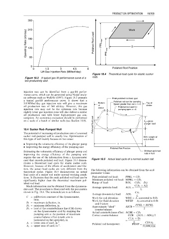
Figure 18.4 Theoretical load cycle for elastic sucker
Figure 18.3 A typical gas lift performance curve of a rods.
low-productivity well.

injection rate can be identified from a gas-lift perfor-
mance curve, which can be generated using Nodal analy-
sis software such as WellFlo (1997). Figure 18.3 presents Peak polished rod load. pprl
a typical gas-lift performance curve. It shows that a Polished rod card for pumping
5.0-MMscf/day gas injection rate will give a maximum Bottom Speed greater than zero. n > 0 Top of
oil production rate of 260 stb/day. However, this gas of Polished rod card for stroke
injection rate may not be the optimum rate because stroke pumping spee. n = 0
slightly lower gas injection rates will also deliver a similar
oil production rate with lower high-pressure gas con- F 1
Polished Rod Load plunger load
sumption. An economics evaluation should be performed
on a scale of a batch of similar wells (see Section 18.9). F 0 = gross

18.4 Sucker Rod–Pumped Well
The potential of increasing oil production rate of a normal F 2
sucker rod–pumped well is usually low. Optimization of Wrf = weight of
this type of well mainly focuses on two areas: rods in fluid
. Improving the volumetric efficiency of the plunger pump s
. Improving the energy efficiency of the pumping unit
Polished Rod Position
Estimating the volumetric efficiency of plunger pump and Minimum polished
improving the energy efficiency of the pumping unit rods in fluid
require the use of the information from a dynamometer
card that records polished rod load. Figure 18.4 demon- Figure 18.5 Actual load cycle of a normal sucker rod.
strates a theoretical load cycle for elastic sucker rods.
However, because of the effects of acceleration and fric-
tion, the actual load cycles are very different from the The following information can be obtained from the card
theoretical cycles. Figure 18.5 demonstrates an actual parameter values:
load cycle of a sucker rod under normal working condi-
tions. It illustrates that the peak polished rod load can be Peak polished rod load: PPRL ¼ CD 1
significantly higher than the theoretical maximum pol- Minimum polished rod load: MPRL ¼ CD 2
ished rod load. Range of load: ROL ¼ C(D 1 D 2 )
Much information can be obtained from the dynamom- Average upstroke load: AUL ¼ CðA 1 þ A2Þ
eter card. The procedure is illustrated with the parameters L
shown in Fig. 18.6. The nomenclature is as follows: CA 1
Average downstroke load: ADL ¼
L
C ¼ calibration constant of the dynamometer, Work for rod elevation: WRE ¼ A 1 converted to ft-lb
lb/in. Work for fluid elevation WFEF ¼ A 2 converted to ft-lb
D 1 ¼ maximum deflection, in. and friction:
D 2 ¼ minimum deflection, in. Approximate ‘‘ideal’’ AICB ¼ PPRL þ MPRL
D 3 ¼ load at the counterbalance line (CB) drawn counterbalance: 2
on the dynamometer card by stopping the
Actual counterbalance effect: ACBE ¼ CD 3
pumping unit at the position of maximum Correct counterbalance: CCB ¼ (AUL þ ADL)=2
counterbalance effect (crank arm is
CA 1 þ A 2 )
horizontal on the upstroke), in. ¼ 2
L
A 1 ¼ lower area of card, in: 2 Polished rod horsepower: PRHP ¼ CSNA 2
2
A 2 ¼ upper area of card, in: . 33,000(12)L