Page 264 - Petroleum Production Engineering, A Computer-Assisted Approach

Guo, Boyun / Computer Assited Petroleum Production Engg 0750682701_chap17 Final Proof page 263 3.1.2007 9:19pm Compositor Name: SJoearun

HYDRAULIC FRACTURING 17/263
Simulating controlled height growth with a pseudo-3D Post-propped Frac Decline. The simulator-generated
model can be tricky. Height growth is characterized by pressure decline is affected by the model of extension
a slower rate of pressure increase than in the case of a recession that is implemented and by the amount of sur-
confined fracture. To capture the big picture, a simplifica- face area that still have leakoff when the simulator cells are
tion to a three-layer model can help by reducing the num- packed with proppant. It is very unlikely that the simula-
ber of possible inputs. Pressure-matching slow height tor matches any of those extreme cases. The lumped solu-
growth of a fracture is tedious and lengthy. In the first tion used in FracProPT does a good job of matching
phase, we should adjust the magnitude of the simulated pressure decline. The analysis methodology was indeed
net pressure. The match can be considered excellent if developed around pressure matching the time to closure.
the difference between the recorded pressure and the The time to closure always relates to the efficiency of the
simulated pressure is less than 15% over the length of fluid regardless of models (Nolte and Smith, 1981).
the pad.
The pressure matching can be performed using data
from real-time measurements (Wright et al., 1996; Burton 17.6.2 Pressure Buildup Test Analysis
et al., 2002). Computer simulation of fracturing operations Fracture and reservoir parameters can be estimated using
with recorded job parameters can yield the following frac- data from pressure transient well tests (Cinco-Ley and
ture dimensions: Samaniego, 1981; Lee and Holditch, 1981). In the pressure
transient well-test analysis, the log-log plot of pressure
. Fracture height derivative versus time is called a diagnostic plot. Special
. Fracture half-length slope values of the derivative curve usually are used
. Fracture width for identification of reservoir and boundary models. The
transient behavior of a well with a finite-conductivity
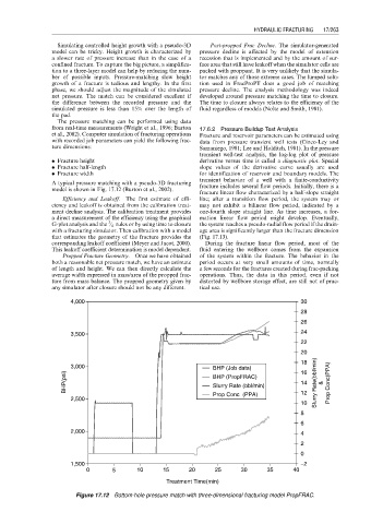
A typical pressure matching with a pseudo-3D fracturing fracture includes several flow periods. Initially, there is a
model is shown in Fig. 17.12 (Burton et al., 2002).
fracture linear flow characterized by a half-slope straight
Efficiency and Leakoff. The first estimate of effi- line; after a transition flow period, the system may or
ciency and leakoff is obtained from the calibration treat- may not exhibit a bilinear flow period, indicated by a
ment decline analysis. The calibration treatment provides one-fourth–slope straight line. As time increases, a for-
a direct measurement of the efficiency using the graphical mation linear flow period might develop. Eventually,
3
G-plot analysis and the ⁄ 4 rules or by using time to closure the system reaches a pseudo-radial flow period if the drain-
with a fracturing simulator. Then calibration with a model age area is significantly larger than the fracture dimension
that estimates the geometry of the fracture provides the (Fig. 17.13).
corresponding leakoff coefficient (Meyer and Jacot, 2000). During the fracture linear flow period, most of the
This leakoff coefficient determination is model dependent. fluid entering the wellbore comes from the expansion
Propped Fracture Geometry. Once we have obtained of the system within the fracture. The behavior in the
both a reasonable net pressure match, we have an estimate period occurs at very small amounts of time, normally
of length and height. We can then directly calculate the a few seconds for the fractures created during frac-packing
average width expressed in mass/area of the propped frac- operations. Thus, the data in this period, even if not
ture from mass balance. The propped geometry given by distorted by wellbore storage effect, are still not of prac-
any simulator after closure should not be any different. tical use.

4,000 30
28
26

3,500 24
22
20
18
3,000 BHP (Job data) 16
BHP(psi) BHP (PropFRAC) 14 Slurry Rate(bbl/min) & Prop Conc(PPA)

Slurry Rate (bbl/min)
Prop Conc (PPA) 12
2,500
10
8
6
2,000
4
2
0
1,500 −2
0 5 10 15 20 25 30 35 40
Treatment Time(min)
Figure 17.12 Bottom-hole pressure match with three-dimensional fracturing model PropFRAC.