Page 261 - Petroleum Production Engineering, A Computer-Assisted Approach

Guo, Boyun / Computer Assited Petroleum Production Engg 0750682701_chap17 Final Proof page 260 3.1.2007 9:19pm Compositor Name: SJoearun

17/260 PRODUCTION ENHANCEMENT
Example Problem 17.4 For Example Problem 17.1, r p ¼ h (17:25)
predict the maximum expected surface injection pressure h f
using the following additional data:
A f ¼ 2x f h f (17:26)
Specific gravity of fracturing fluid: 1.2
Viscosity of fracturing fluid: 20 cp V frac
Tubing inner diameter: 3.0 in. h ¼ (17:27)
V inj
Fluid injection rate: 10 bpm
1 h
Solution V pad ¼ V inj 1 þ h (17:28)
Hydrostatic pressure drop:
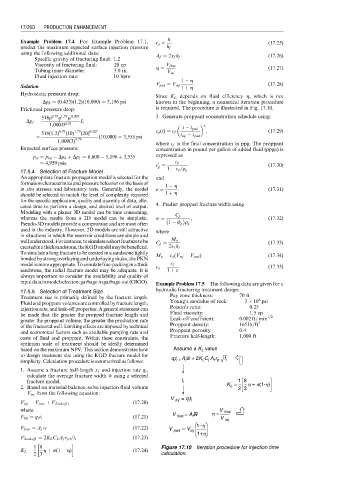
Since K L depends on fluid efficiency h, which is not
Dp h ¼ (0:433)(1:2)(10,000) ¼ 5,196 psi known in the beginning, a numerical iteration procedure
Frictional pressure drop: is required. The procedure is illustrated in Fig. 17.10.
518r 0:79 1:79 m 0:207 3. Generate proppant concentration schedule using:
q
Dp f ¼ L
1,000D 4:79 «
t t pad , (17:29)
518(1:2) 0:79 (10) 1:79 (20) 0:207 c p (t) ¼ c f
¼ (10,000) ¼ 3,555 psi t inj t pad
1,000(3) 4:79
where c f is the final concentration in ppg. The proppant
Expected surface pressure: concentration in pound per gallon of added fluid (ppga) is
p si ¼ p bd Dp h þ Dp f ¼ 6,600 5,196 þ 3,555 expressed as
¼ 4,959 psia c ¼ c p (17:30)
0
p
17.5.4 Selection of Fracture Model 1 c p =r p
An appropriate fracture propagation model is selected for the and
formationcharacteristicsandpressurebehavioronthebasisof 1 h
in situ stresses and laboratory tests. Generally, the model « ¼ : (17:31)
should be selected to match the level of complexity required 1 þ h
for the specific application, quality and quantity of data, allo-
cated time to perform a design, and desired level of output. 4. Predict propped fracture width using
Modeling with a planar 3D model can be time consuming,
whereas the results from a 2D model can be simplistic. w ¼ C p , (17:32)
Pseudo-3D models provide a compromise and are most often 1 f p r p
used in the industry. However, 2D models are still attractive where
in situations in which the reservoir conditions are simple and
wellunderstood.Forinstance,tosimulateashortfracturetobe C p ¼ M p (17:33)
createdinathicksandstone,theKGDmodelmaybebeneficial. 2x f h f
To simulate a long fracture to be created in a sandstone tightly M p ¼ c p (V inj V pad ) (17:34)
c
bondedbystrongoverlayingandunderlayingshales,thePKN
modelismoreappropriate.Tosimulatefrac-packinginathick c p ¼ c f (17:35)
c
sandstone, the radial fracture model may be adequate. It is 1 þ «
always important to consider the availability and quality of
inputdatainmodelselection:garbage-ingarbage-out(GIGO).
Example Problem 17.5 The following data are given for a
hydraulic fracturing treatment design:
17.5.5 Selection of Treatment Size
Pay zone thickness: 70 ft
Treatment size is primarily defined by the fracture length.
6
Young’s modulus of rock: 3 10 psi
Fluid and proppant volumes are controlled by fracture length,
Poison’s ratio: 0.25
injectionrate,andleak-off properties.Ageneralstatementcan
Fluid viscosity: 1.5 cp
be made that the greater the propped fracture length and
Leak-off coefficient: 0:002 ft= min 1=2
greater the proppant volume, the greater the production rate 3
of the fractured well. Limiting effects are imposed by technical Proppant density: 165 lb=ft
and economical factors such as available pumping rate and Proppant porosity: 0.4
costs of fluid and proppant. Within these constraints, the Fracture half-length: 1,000 ft
optimum scale of treatment should be ideally determined
based on the maximum NPV. This section demonstrates how Assume a K value
L
to design treatment size using the KGD fracture model for q t A w + 2K C A r t
simplicity. Calculation procedure is summarized as follows: i i = f L L f p i
1. Assume a fracture half-length x f and injection rate q i ,
calculate the average fracture width w using a selected
w
fracture model. t i 1 8
L
2. Based on material balance, solve injection fluid volume K = 2 3 h + p(1-h)
V inj from the following equation:
V inj = q t i i
V inj ¼ V frac þ V Leakoff , (17:20)
where V = A w h = V frac
V inj ¼ q i t i (17:21) frac f
V inj
w
V frac ¼ A f w (17:22) V pad = V inj 1−h
p ffiffiffi 1+h
V Leakoff ¼ 2K L C L A f r p t i (17:23)

1 8 Figure 17.10 Iteration procedure for injection time
K L ¼ h þ p(1 h) (17:24)
2 3 calculation.