Page 257 - Petroleum Production Engineering, A Computer-Assisted Approach

Guo, Boyun / Computer Assited Petroleum Production Engg 0750682701_chap17 Final Proof page 256 3.1.2007 9:19pm Compositor Name: SJoearun

17/256 PRODUCTION ENHANCEMENT
Planar 3D models: The geometry of a hydraulic fracture is Table 17.1 summarizes main features of fracture models
defined by its width and the shape of its periphery (i.e., height in different categories. Commercial packages are listed in
at any distance from the well and length). The width distri- Table 17.2.
bution and the overall shape change as the treatment is
pumped, and during closure. They depend on the pressure
distribution, which itself is determined by the pressure gra-
dients caused by the fluid flow within the fracture. The 17.4 Productivity of Fractured Wells
relation between pressure gradient and flow rate is very Hydraulically created fractures gather fluids from reser-
sensitive to fracture width, resulting in a tightly coupled voir matrix and provide channels for the fluid to flow into
calculation. Although the mechanics of these processes can wellbores. Apparently, the productivity of fractured wells
be described separately, this close coupling complicates the depends on two steps: (1) receiving fluids from formation
solution of any fracture model. The nonlinear relation be- and (2) transporting the received fluid to the wellbore.
tween width and pressure and the complexity of a moving- Usually one of the steps is a limiting step that controls
boundary problem further complicate numerical solutions. the well-production rate. The efficiency of the first step
Clifton and Abou-Sayed (1979) reported the first numerical depends on fracture dimension (length and height), and
implementation of a planar model. The solution starts with a the efficiency of the second step depends on fracture per-
small fracture, initiated at the perforations, divided into a meability. The relative importance of each of the steps can
number of equal elements (typically 16 squares). The ele- be analyzed using the concept of fracture conductivity
ments then distort to fit the evolving shape. The elements defined as (Argawal et al., 1979; Cinco-Ley and Sama-
can develop large aspect ratios and very small angles, which niego, 1981):
are not well handled by the numerical schemes typically k f w
used to solve the model. Barree (1983) developed a model F CD ¼ , (17:10)
kx f
that does not show grid distortion. The layered reservoir is
divided into a grid of equal-size rectangular elements, over where
the entire region that the fracture may cover. F CD ¼ fracture conductivity, dimensionless
Simulators based on such models are much more com- k f ¼ fracture permeability, md
putationally demanding than P3D-based simulators, be- w ¼ fracture width, ft
cause they solve the fully 2D fluid-flow equations and x f ¼ fracture half-length, ft.
couple this solution rigorously to the elastic-deformation
equations. The elasticity equations are also solved more
rigorously, using a 3D solution rather than 2D slices.
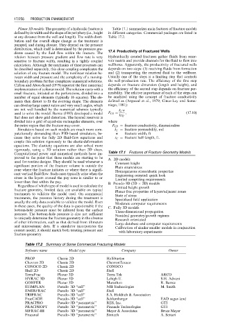
Computational power and numerical methods have im- Table 17.1 Features of Fracture Geometry Models
proved to the point that these models are starting to be A. 2D models
used for routine designs. They should be used whenever a Constant height
significant portion of the fracture volume is outside the Plain strain/stress
zone where the fracture initiates or where there is signifi- Homogeneous stress/elastic properties
cant vertical fluid flow. Such cases typically arise when the Engineering oriented: quick look
stress in the layers around the pay zone is similar to or Limited computing requirements
lower than that within the pay. B. Pseudo-3D (2D 2D) models
Regardless of which type of model is used to calculate the Limited height growth
fracture geometry, limited data are available on typical Planar frac properties of layers/adjacent zones
treatments to validate the model used. On commercial State of stress
treatments, the pressure history during the treatment is Specialized field application
usually the only data available to validate the model. Even Moderate computer requirements
in these cases, the quality of the data is questionable if the C. Fully 3D models
bottom-hole pressure must be inferred from the surface Three-dimensional propagation
pressure. The bottom-hole pressure is also not sufficient Nonideal geometry/growth regimes
to uniquely determine the fracture geometry in the absence Research orientated
of other information, such as that derived from tiltmeters Large database and computer requirements
and microseismic data. If a simulator incorporates the Calibration of similar smaller models in conjunction
correct model, it should match both treating pressure and with laboratory experiments
fracture geometry.
Table 17.2 Summary of Some Commercial Fracturing Models
Software name Model type Company Owner
PROP Classic 2D Halliburton
Chevron 2D Classic 2D ChevronTexaco
CONOCO 2D Classic 2D CONOCO
Shell 2D Classic 2D Shell
TerraFrac Planar 3D Terra Tek ARCO
HYRAC 3D Planar 3D Lehigh U. S.H. Advani
GOHFER Planar 3D Marathon R. Barree
STIMPLAN Pseudo–3D ‘‘cell’’ NSI Technologies M. Smith
ENERFRAC Pseudo–3D ‘‘cell’’ Shell
TRIFRAC Pseudo–3D ‘‘cell’’ S.A. Holditch & Association
FracCADE Pseudo–3D ‘‘cell’’ Schlumberger EAD sugar-land
PRACPRO Pseudo–3D ‘‘parametric’’ RES, Inc. GTI
PRACPROPT Pseudo–3D ‘‘parametric’’ Pinnacle Technologies GTI
MFRAC-III Pseudo–3D ‘‘parametric’’ Meyer & Associates Bruce Meyer
Fracanal Pseudo–3D ‘‘parametric’’ Simtech A. Settari