Page 256 - A First Course In Stochastic Models

POLICY-ITERATION ALGORITHM 249

∗
unit. It is stated without proof that the function υ , i ∈ I, in (6.4.3) is uniquely
i
determined up to an additive constant.
Next the policy-iteration algorithm is applied to compute an average cost optimal
policy for the control problem in Example 6.1.1.
Example 6.1.1 (continued) A maintenance problem

It is assumed that the number of possible working conditions equals N = 5. The
repair costs are given by C f = 10, C p2 = 7, C p3 = 7 and C p4 = 5. The deteri-
oration probabilities q ij are given in Table 6.4.1. The policy-iteration algorithm is
initialized with the policy R (1) = (0, 0, 0, 0, 2, 2), which prescribes repair only in
the states 5 and 6. In the calculations below, the policy-improvement quantity is
abbreviated as

T i (a, R) = c i (a) − g(R) + p ij (a)v j (R)
j∈I

when the current policy is R. Note that always T i (a, R) = v i (R) for a = R i .
Iteration 1
Step 1 (value determination). The average cost and the relative values of policy
R (1) = (0, 0, 0, 0, 2, 2) are computed by solving the linear equations

v 1 = 0 − g + 0.9v 1 + 0.1v 2

v 2 = 0 − g + 0.8v 2 + 0.1v 3 + 0.05v 4 + 0.05v 5
v 3 = 0 − g + 0.7v 3 + 0.1v 4 + 0.2v 5
v 4 = 0 − 9 + 0.5v 4 + 0.5v 5
v 5 = 10 − g + v 6
v 6 = 0 − g + v 1
v 6 = 0,

where state s = 6 is chosen for the normalizing equation v s = 0. The solution of
these linear equations is given by
(1) (1) (1) (1)
g(R ) = 0.5128, v 1 (R ) = 0.5128, v 2 (R ) = 5.6410, v 3 (R ) = 7.4359,
(1) (1) (1)
v 4 (R ) = 8.4615, v 5 (R ) = 9.4872, v 6 (R ) = 0.

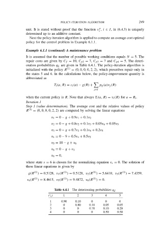
Table 6.4.1 The deteriorating probabilities q ij
i\j 1 2 3 4 5
1 0.90 0.10 0 0 0
2 0 0.80 0.10 0.05 0.05
3 0 0 0.70 0.10 0.20
4 0 0 0 0.50 0.50