Page 259 - A First Course In Stochastic Models

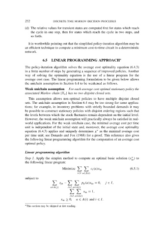
252 DISCRETE-TIME MARKOV DECISION PROCESSES

(d) The relative values for transient states are computed first for states which reach
the cycle in one step, then for states which reach the cycle in two steps, and
so forth.

It is worthwhile pointing out that the simplified policy-iteration algorithm may be
an efficient technique to compute a minimum cost-to-time circuit in a deterministic
network.

6.5 LINEAR PROGRAMMING APPROACH ∗
The policy-iteration algorithm solves the average cost optimality equation (6.4.3)
in a finite number of steps by generating a sequence of improved policies. Another
way of solving the optimality equation is the use of a linear program for the
average cost case. The linear programming formulation to be given below allows
the unichain assumption in Section 6.4 to be weakened as follows.
Weak unichain assumption For each average cost optimal stationary policy the
associated Markov chain {X n } has no two disjoint closed sets.
This assumption allows non-optimal policies to have multiple disjoint closed
sets. The unichain assumption in Section 6.4 may be too strong for some applica-
tions; for example, in inventory problems with strictly bounded demands it may
be possible to construct stationary policies with disjoint ordering regions such that
the levels between which the stock fluctuates remain dependent on the initial level.
However, the weak unichain assumption will practically always be satisfied in real-
world applications. For the weak unichain case, the minimal average cost per time
unit is independent of the initial state and, moreover, the average cost optimality
equation (6.4.3) applies and uniquely determines g as the minimal average cost
∗
per time unit; see Denardo and Fox (1968) for a proof. This reference also gives
the following linear programming algorithm for the computation of an average cost
optimal policy.

Linear programming algorithm
Step 1. Apply the simplex method to compute an optimal basic solution (x ) to
∗
ia
the following linear program:

Minimize c i (a)x ia (6.5.1)
i∈I a∈A(i)
subject to

x ja − p ij (a)x ia = 0, j ∈ I,
a∈A(j) i∈I a∈A(i)

x ia = 1,
i∈I a∈A(i)
x ia ≥ 0, a ∈ A(i) and i ∈ I.
∗ This section may be skipped at first reading.