Page 257 - A First Course In Stochastic Models

250 DISCRETE-TIME MARKOV DECISION PROCESSES

Step 2 (policy improvement). The test quantity T i (a, R) has the values

T 2 (0, R (1) ) = 5.6410, T 2 (1, R (1) ) = 7.0000, T 3 (0, R (1) ) = 7.4359,

T 3 (1, R (1) ) = 7.0000, T 4 (0, R (1) ) = 9.4872, T 4 (1, R (1) ) = 5.0000.
This yields the new policy R (2) = (0, 0, 1, 1, 2, 2) by choosing for each state i the
action a that minimizes T i (a, R (1) ).
Step 3 (convergence test). The new policy R (2) is different from the previous policy
R (1) and hence another iteration is performed.
Iteration 2
Step 1 (value determination). The average cost and the relative values of policy
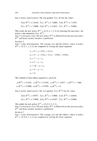
R (2) = (0, 0, 1, 1, 2, 2) are computed by solving the linear equations

v 1 = 0 − g + 0.9v 1 + 0.1v 2

v 2 = 0 − g + 0.8v 2 + 0.1v 3 + 0.05v 4 + 0.05v 5
v 3 = 7 − g + v 1
v 4 = 5 − g + v 1
v 5 = 10 − g + v 6
v 6 = 0 − g + v 1
v 6 = 0.

The solution of these linear equations is given by

g(R (2) ) = 0.4462, v 1 (R (2) ) = 0.4462, v 2 (R (2) ) = 4.9077, v 3 (R (2) ) = 7.000,
(2) (2) (2)
v 4 (R ) = 5.0000, v 5 (R ) = 9.5538, v 6 (R ) = 0.
Step 2 (policy improvement). The test quantity T i (a, R (2) ) has the values

T 2 (0, R (2) ) = 4.9077, T 2 (1, R (2) ) = 7.0000, T 3 (0, R (2) ) = 6.8646,
T 3 (1, R (2) ) = 7.0000, T 4 (0, R (2) ) = 6.8307, T 4 (1, R (2) ) = 5.0000.

This yields the new policy R (3) = (0, 0, 0, 1, 2, 2).
Step 3 (convergence test). The new policy R (3) is different from the previous policy
R (2) and hence another iteration is performed.
Iteration 3
Step 1 (value determination). The average cost and the relative values of policy
R (3) = (0, 0, 0, 1, 2, 2) are computed by solving the linear equations