Page 258 - A First Course In Stochastic Models

POLICY-ITERATION ALGORITHM 251

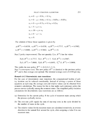
v 1 = 0 − g + 0.9v 1 + 0.1v 2
v 2 = 0 − g + 0.8v 2 + 0.1v 3 + 0.05v 4 + 0.05v 5

v 3 = 0 − g + 0.7v 3 + 0.1v 4 + 0.2v 5
v 4 = 5 − g + v 1
v 5 = 10 − g + v 6
v 6 = 0 − g + v 1
v 6 = 0.

The solution of these linear equations is given by

g(R (3) ) = 0.4338, v 1 (R (3) ) = 0.4338, v 2 (R (3) ) = 4.7717, v 3 (R (3) ) = 6.5982,
v 4 (R (3) ) = 5.0000, v 5 (R (3) ) = 9.5662, v 6 (R (3) ) = 0.

Step 2 (policy improvement). The test quantity T i (a, R (3) ) has the values

T 2 (0, R (3) ) = 4.7717, T 2 (1, R (3) ) = 7, T 3 (0, R (3) ) = 6.5987,
T 3 (1, R (3) ) = 7.0000, T 4 (0, R (3) ) = 6.8493, T 4 (1) (1, R (3) ) = 5.0000.

This yields the new policy R (4) = (0, 0, 0, 1, 2, 2).
Step 3 (convergence test). The new policy R (4) is identical to the previous policy
R (3) and is thus average cost optimal. The minimal average cost is 0.4338 per day.

Remark 6.4.2 Deterministic state transitions
For the case of deterministic state transitions the computational burden of pol-
icy iteration can be reduced considerably. Instead of solving a system of linear
equations at each step, the average cost and relative values can be obtained from
recursive calculations. The reason for this is that under each stationary policy the
process moves cyclically among the recurrent states. The simplified policy-iteration
calculations for deterministic state transitions are as follows:

(a) Determine for the current policy R the cycle of recurrent states among which
the process cyclically moves.
(b) The cost rate g(R) equals the sum of one-step costs in the cycle divided by
the number of states in the cycle.
(c) The relative values for the recurrent states are calculated recursively, in reverse
direction to the natural flow around the cycle, after assigning a value 0 to one
recurrent state.