Page 262 - A First Course In Stochastic Models

LINEAR PROGRAMMING APPROACH 255

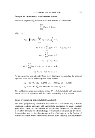
Example 6.1.1 (continued) A maintenance problem
The linear programming formulation for this problem is to minimize

N−1

C pi x i1 + C f x N2
i=2
subject to

N−1

x 10 − q 11 x 10 + x i1 + x N+1,2 = 0,
i=2
j

x j0 + x j1 − q ij x i0 = 0, 2 ≤ j ≤ N − 1,
i=1
N−1

x N2 − q iN x i0 = 0,
i=1
x N+1,2 − x N2 = 0,
N−1

x 10 + (x i0 + x i1 ) + x N2 + x N+1,2 = 1,
i=2
x 10 , x i0 , x i1 , x N2 , x N+1,2 ≥ 0.

For the numerical data given in Table 6.4.1, this linear program has the minimal
objective value 0.4338 and the optimal basic solution

∗
x 10 = 0.5479, x ∗ 20 = 0.2740, x ∗ 30 = 0.0913, x 41 = 0.0228,
∗
∗
∗
x 52 = 0.0320, x ∗ 62 = 0.0320 and the other x = 0.
ia
This yields the average cost optimal policy R = (0, 0, 0, 1, 2, 2) with an average
∗
cost of 0.4338, in agreement with the results obtained by policy iteration.
Linear programming and probabilistic constraints
The linear programming formulation may often be a convenient way to handle
Markovian decision problems with probabilistic constraints. In many practical
applications, constraints are imposed on certain state frequencies. For example,
in inventory problems for which shortage costs are difficult to estimate, probabilis-
tic constraints may be placed on the probability of shortage or on the fraction of
demand that cannot be met directly from stock on hand. Similarly, in a maintenance