Page 15 - A Practical Companion to Reservoir Stimulation

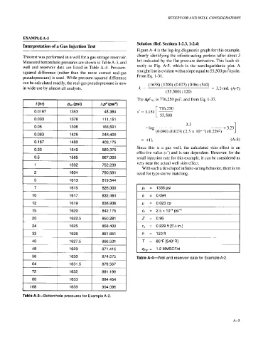
RESERVOIR AND WELL CONSIDERATIONS

EXAMPLE A-2
Solution (Ref. Sections 1-2.3,l-2.4)
Interpretation of a Gas Injection Test
Figure A-4 is the log-log diagnostic graph for this example,
This test was performed in a well for a gas storage reservoir. clearly identifying the infinite-acting portion (after about 3
Measured bottomhole pressures are shown in Table A-3, and hr) indicated by the flat pressure derivative. This leads di-
well and reservoir data are listed in Table A-4. Pressure- rectly to Fig. A-5, which is the semilogarithmic plot. A
squared difference (rather than the more correct real-gas straight line is evident with a slope equal to 55,500 psi?/cycle.
pseudopressure) is used. While pressure-squared difference From Eq. 1-3 1,
can be calculated readily, the real-gas pseudopressure is now ( 1638) ( 1200) (0.023) (0.96) (540)
in wide use by almost all analysts. k= = 3.5 md. (A-7)
(55,500) (120)
The A$,,,,- is 776,250 psi?, and from Eq. 1-37,
[ :goo
0.0167 48,384 s'= 1.151 ~
0.033 11 1,151
3.5 1
166,591 - log + 3.23
I 0.083 I 1425 I 248,400 (0.094) (0.023) (2.5 x 10-4)(0.229')
I 0.167 I 1480 I 408,175 = +11. ('4-8)

Since this is a gas well, the calculated skin effect is an
589,375
effective value (s') and is rate dependent. However, for the
667,000 small injection rate for this example, it can be considered as
very near the actual well skin effect.
1592 752,239 With such a developed infinite-acting behavior, there is no
I I
1 2 1604 790,591 need for type-curve matching.
I I
1 5 1613 819,544
826,000
832,464 4 = 0.094
838,936 0.023 cp
I l5 I 1620 I 842,175 I c, = 2.5 x 10-4 psi-' 1
I 20 I 1622.5 I 850,281 I Z = 0.96 1

858,400 I r, = 0.229 ft [5% in.] 1
861,651 h = 120ft
40 1627.5 866,53 1 T = 80°F [540"R]
I 48 I 1629 I 871,416 I = 1.2 MMSCF/d 1

56 1630 874,675 Table A-4-Well and reservoir data for Example A-2.
64 1631.5 879,567
72 1632 881,199
80 1633 884,464
I 168 I 1639 I 904,096

Table A-3-Bottomhole pressures for Example A-2.

A- 5