Page 56 - A Practical Companion to Reservoir Stimulation

PRACTICAL COMPANION TO RESERVOIR STIMULATION

EXAMPLE D-4
From Eq. D- 1 1 and using the variables in Table D-3, the
Calculation of Fracture Penetration constant CI can be calculated:
and Net Pressure Increase vs. Time
C, = (0.589) (0.4395) (0.00753)
Develop the relationships that would provide the fracture = 1.95 x lo.? (D-16)
penetration and net pressure increase for the PKN model
(q = 1). Apply this calculation to the reservoir with the From Eq. D- 13,
variables in Table D-3.
X, = 559.4t075, (D-17)
Solution (Ref. Sections 3-3.43 and 7-3) where .t is in minutes.
For q + 1, from Eqs. 7-37 and 7-40 for the PKN model, From Eq. D-15,

qit
x, = -. (D- 10) Apr = 53.; 333. (D-18)
2hJw
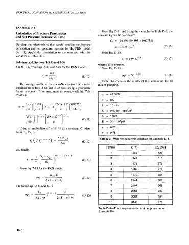
Table D-4 contains the results of this simulation for 10
The average width, w, for a non-Newtonian fluid can be min of pumping.
obtained from Eqs. 3-62 and 3-72 (and using a geometric
factor to convert from maximum to average width). This
results in qi = 40BPM
n’ = 0.5
t = 10rnin
K = 0.02 Ibf - secn‘lft2
hf = l00ft
(D-1 1)
E = 3 x 106psi

Using all multipliers of ~f1’(~~’ as a constant, CI, then v = 0.25
2,
from Eq. D-10, + y = 0.75
( X~/(2n’ + 2)) 5.6 15 q, t Table D-%Well and reservoir variables for Example D-4.
’1 I f - (D-12)
2hJ ’
and finally
(2n’ + 2)/(2n’ + 3)
5.615q,t
1
x/ =- Cl [F]’ (D- 13)
From Eq. 7- 13 for the PKN model,

(D-14)

and from Eqs. D- 1 1 and D- 12

(D-15)

Table D-4-Fracture penetration and net pressure for
Example D-4.

D-6