Page 61 - A Practical Companion to Reservoir Stimulation

E. Design and Modeling of Propped Fractures

EXAMPLE E-1
and finally, from Eq. 8-9,
Calculation of Transient IPR Curves
[
(
PKf ] - 0.8 ( pwf 71. (E-5)
Calculate transient inflow performance relationships (IPR) 9 z.245 + 400 1 - 0.2 - 4700
4700
~
for 10 days, 30 days and 365 days using the data given in
Table E-I. Use bottomhole pressures, above and below the For t = 30 days, the tDXf = 5.5 x andp, (from Fig. 8-2)
bubblepoint pressure. is 0.23. Then, from Eq. 8-6, qh= 160 STB/d, and from
Eqs. 8-7 and 8-8, qvon,l = 261 STB/d. Finally, from Eq. 8-9,
Solution (Ref. Section 8-2.1)
From Eq. 8-5, ) ,’I.
q = 160 + 261 [ 1 - 0.2 ( - 0.8 ( - (E-6)
pwf
pd
-
750 4700 4700
FCD = = 10.
(0.05) (1500) Fort = 365 days, tDxf = 6.7 x lo-* andp, (from Fig. 8-2) is
0.6. Then, from Eq. 8-6, qb = 61 STB/d, and from Eqs. 8-7
Since A = 320 acres, the side of the square is 3734 ft, and
the reservoir half-length is 1867 ft, which can contain the and 8-8, qVogel = 100 STB/d. From Eq. 8-9,
designed fracture half-length. Thus, Fig. 8-2 for FcD = 10 can
[
( pwf ) - 0.8 ( - 71. (E-7)
be used for the forecast. = 61 + 100 1 - 0.2 - pwf
Fort = 10 days, the dimensionless time can be calculated 4700 4700
from Eq. 8-3: Figure E- 1 contains the standard q vs. p,,,fplots for the three
(0.000264) (0.05) ( 10) (24) transient IPRs as calculated from Eqs. E-5, E-6 and E-7.
IDXf = (0.1 1) (0.7) ( ( 1500)2

= 1.83 x (E-2) I k = 0.05md 1
From Fig. 8-2, pD = 0.15, and from Eq. 8-6, the flow rate,
if the flowing bottomhole pressure is the bubblepoint pres-
sure, can be calculated:
(0.05) (50) (6300 - 4700) 1
qb = = 245STB/d. (E-3) q3 = 0.11
(141.2) (1.1) (0.7) (0.15) 1
A = 320acres
From Eqs. 8-7 and 8-8,
(245) (4700)
qvl,g,Ke/ = = 400STB/d, (E-4)
(6300 - 4700) ( 1.8)
1
I k,w = 750 md-ft

I /Ao = 0.7cp 1
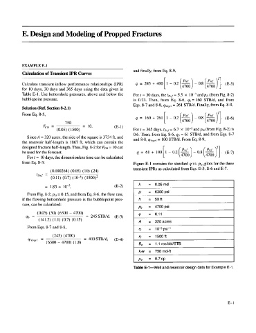
Table E-1-Well and reservoir design data for Example E-I.

E- 1