Page 63 - A Practical Companion to Reservoir Stimulation

DESIGN AND MODELING OF PROPPED FRACTURES

EXAMPLE E-2
From Eq. 8-3 and for t = 365 days, rDxf= 0.6 (for xf= 500
IPR Curves with x,Variation
ft), and toX,f= 0.15 (for xt= 1000 ft). Then, from Fig. 8-2,
p~ = 0.8 (for 500 ft), and pD = 0.65 (for 1000 ft).
Construct transient IPR curves for the 1-yr time for fracture From Eq. 8-6, qb is then 46 STB/d (for 500 ft) and 57
half-lengths equal to 500 and 1000 ft. Use all other variables STB/d (for 1000 ft).
as in Example E- I. From Eqs. 8-6 and 8-8, qw,gr, is 75 STB/d and 93 STB/d,

Solution (Ref. Section 8-2.1) respectively. Finally, from Eq. 8-9,
For this example the FcD value is different for each fracture
length. (It assumes that kpv is constant. In reality, this cannot =,46 + 75 [ 1 - 0.2 ( - pwf ) - 0.8 (’” - 71 (E-10)
be so because w is a function of xf However, for the purposes 4700 4700
of this exercise, kfw = 750 md-ft.) for xf= 500 ft, and
For xs= 500 ft,
)2]
)
750 = 57 + 93 [ 1 - 0.2 (’” - 0.8 ( - (E-11)
pwf
-
Fcr, = = 30, (E-8) 4700 4700
(0.05) (500)
for .xr = 1000 ft.
and for q = 1000 ft ,
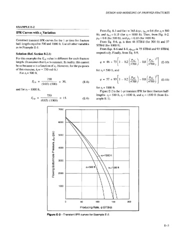
Figure E-2 is the I-yr transient IPR for three fracture half-
750 lengths: xf= 500 ft, xf= 1000 ft, and xr= 1500 ft (from Ex-
Fcu = = 15. (E-9) ample E- 1 ).
(0.05) (1000)

7000

6000

i=-
v)
5000
L
d
n!
=I
$ 4000
F
a
a, -
0
c
5 3000
E:
0
m
0)
.- 2000
K
6
iT
1000

0 50 100 150 200
Producing Rate, 9 (STB/d)

Figure E-2-Transient IPR curves for Example E-2.

E-3