Page 67 - A Practical Companion to Reservoir Stimulation

DESIGN AND MODELING OF PROPPED FRACTURES

EXAMPLE E-4
In the right side of Eq. E- 15, the two parentheses denote the
Calculation of Fracture Width
maximum width (at the wellbore) and the PKN geometric
factor. The product of the two is the average fracture width.
Calculate the average fracture width of a 1 000-ft fracture half- In order to calculate the width with the KGD model, Eq.
length for a Newtonian fluid. Repeat the calculation for a 8-21 with coherent units is transformed into
range of fractures from 100 ft to 500 ft for both the PKN and
the KGD models. Use the data in Table E-3.

Solution (Ref. 8-2.4)
The width for the PKN model (which is the appropriate one
for this problem sincexf” hf) is given by Eq. 8- 19 in coherent for the common units in Table E-3. Figure E-5 is a graph of
units. For the common units, listed in Table E-3, Eq. 8-19 the average width for the two models for a range of fracture
becomes: half-lengths from 100 to 500 ft.
As can be seen easily from Eqs. E- 12 and E- 16, control of
the fracture width during execution is not accomplished eas-
(E-12) ily. To double the width for a given reservoir (i.e., given V, E
and hf) at a desired fracture length would require an increase
with the width, w, in inches. of the product qip by a factor of 16. Because the viscosity is
The elastic shear modulus is given by associated with undesirable side effects such as residual
proppant-pack damage, increasing the rate is the remaining
E means of width control. For this problem, doubling the rate to
G= (E- 13)
2(1 + v)’ 80 BPM (this would have an impact on treating pressure and
fracture height migration) would increase the average width
and therefore, for this problem,
by a factor of 2°.25, or 1.2 (i.e., by 20%).
3 x lo6
G= = 1.2 x lo6. (E-14)
2 (I + 0.25)
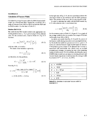
From Eq. E- 12, I q = 40BPM I
h, = 100ft
I
(40) ( 100) (0.75) ( 1000)
[ 1.2 x 106
w = 0.3 1 4 [; 0.75) E = 3 x 106psi
= (0.38) (0.59) = 0.22in. (E- 15) I ji = 1oocp I
I y = 0.75 I

Table E-3-Variables to calculate fracture width for
Example E-4.

E-7