Page 344 - Accounting Information Systems

C H A P TER 7 The Conversion Cycle 315

FI G U R E
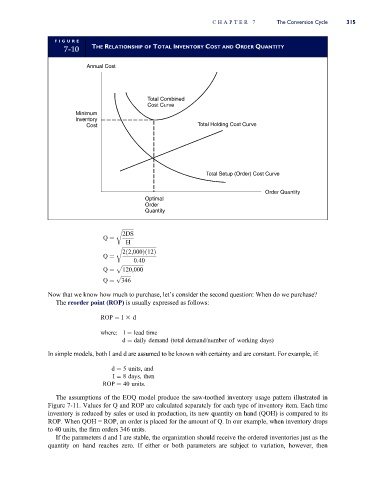
7-10 THE RELATIONSHIP OF TOTAL INVENTORY COST AND ORDER QUANTITY

Annual Cost

Total Combined
Cost Curve
Minimum
Inventory
Cost Total Holding Cost Curve

Total Setup (Order) Cost Curve

Order Quantity
Optimal
Order
Quantity

r ffiffiffiffiffiffiffiffiffi
2DS
Q ¼
H
r ffiffiffiffiffiffiffiffiffiffiffiffiffiffiffiffiffiffiffiffiffiffiffiffiffiffi
2ð2;000Þð12Þ
Q ¼
0:40
p ffiffiffiffiffiffiffiffiffiffiffiffiffiffiffiffi
Q ¼ 120;000
p ffiffiffiffiffiffiffiffi
Q ¼ 346
Now that we know how much to purchase, let’s consider the second question: When do we purchase?
The reorder point (ROP) is usually expressed as follows:

ROP ¼ I 3 d
where: I ¼ lead time
d ¼ daily demand (total demand/number of working days)
In simple models, both I and d are assumed to be known with certainty and are constant. For example, if:

d ¼ 5 units, and
I ¼ 8 days, then
ROP ¼ 40 units.
The assumptions of the EOQ model produce the saw-toothed inventory usage pattern illustrated in
Figure 7-11. Values for Q and ROP are calculated separately for each type of inventory item. Each time
inventory is reduced by sales or used in production, its new quantity on hand (QOH) is compared to its
ROP. When QOH = ROP, an order is placed for the amount of Q. In our example, when inventory drops
to 40 units, the firm orders 346 units.
If the parameters d and I are stable, the organization should receive the ordered inventories just as the
quantity on hand reaches zero. If either or both parameters are subject to variation, however, then