Page 288 - Acquisition and Processing of Marine Seismic Data

5.6 GAIN RECOVERY 279

P
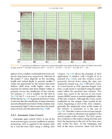
FIG. 5.39 t corrections for different P values on a marine shot gather from relatively deeper waters. (A) Filtered shot with
P
no gain, and its t corrected versions for (B) P ¼ 1.0, (C) P ¼ 2.0, (D) P ¼ 4.0, (E) P ¼ 6.0, and (F) P ¼ 10.0.
gathers from a shallow continental shelf and a rel- window. Fig. 5.40 shows the principle of AGC
atively deep basin area, respectively. Selection of application. A window with a length of Δt is
the proper P value depends on the recording selected (Fig. 5.40A), and this window is pro-
length and seabed depth. In general, smaller P gressively moved down along the time axis
values are appropriate for the seismic data from sample-by-sample (e.g., Fig. 5.40B and C). Here,
shallow shelf areas while higher values are Δt is also known as AGC operator length. Each
required for seismic data from deeper waters, to time, a scale factor is calculated using the ampli-
properly recover the amplitudes of late arrivals. tudes within the specified time window. This
For instance, P ¼ 2.0 is suitable for the shot in scalar may equal to the inverse of root mean
Fig. 5.38,but P ¼ 4oreven P ¼ 6can be selected square (RMS), mean or median amplitude value
fortheshotinFig.5.39.Ingeneral,ifalowerPvalue of the time window. Although the scalar can be
is selected, then the amplitudes of deep reflections multiplied by the sample value located at the
arenotsufficientlyrecovered.Onthecontrary,ifan center, beginning or end of the AGC window,
unnecessarily high P value is used, then the ampli- generally the amplitude value at the center of
tudes of early arrivals almost die (Fig. 5.38F). the window is preferred, as is the case in
Fig. 5.40. Then the window is moved one sample
and a new scalar is calculated and applied to the
5.6.3 Automatic Gain Control
central sample of the window. The AGC opera-
Automatic gain control (AGC) is one of the tion continues in this fashion along the time axis
most common gain recovery methods in seismic from the beginning to the end of the time sam-
processing. AGC is applied to the seismic data ples within the trace. At the beginning and
on a trace-by-trace basis using a sliding time end of the trace, however, there will not be