Page 289 - Acquisition and Processing of Marine Seismic Data

280 5. PREPROCESSING

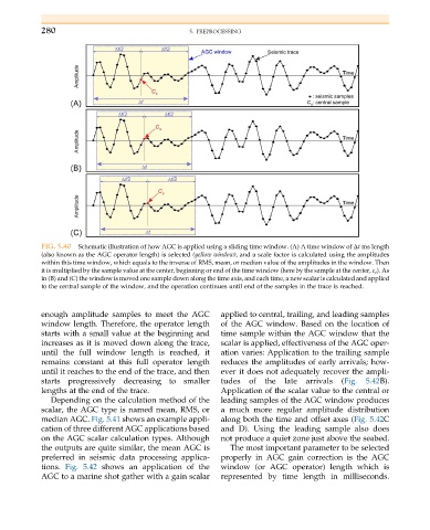
FIG. 5.40 Schematic illustration of how AGC is applied using a sliding time window. (A) A time window of Δt ms length
(also known as the AGC operator length) is selected (yellow window), and a scale factor is calculated using the amplitudes
within this time window, which equals to the inverse of RMS, mean, or median value of the amplitudes in the window. Then
it is multiplied by the sample value at the center, beginning or end of the time window (here by the sample at the center, c s ). As
in (B) and (C) the window is moved one sample down along the time axis, and each time, a new scalar is calculated and applied
to the central sample of the window, and the operation continues until end of the samples in the trace is reached.

enough amplitude samples to meet the AGC applied to central, trailing, and leading samples
window length. Therefore, the operator length of the AGC window. Based on the location of
starts with a small value at the beginning and time sample within the AGC window that the
increases as it is moved down along the trace, scalar is applied, effectiveness of the AGC oper-
until the full window length is reached, it ation varies: Application to the trailing sample
remains constant at this full operator length reduces the amplitudes of early arrivals; how-
until it reaches to the end of the trace, and then ever it does not adequately recover the ampli-
starts progressively decreasing to smaller tudes of the late arrivals (Fig. 5.42B).
lengths at the end of the trace. Application of the scalar value to the central or
Depending on the calculation method of the leading samples of the AGC window produces
scalar, the AGC type is named mean, RMS, or a much more regular amplitude distribution
median AGC. Fig. 5.41 shows an example appli- along both the time and offset axes (Fig. 5.42C
cation of three different AGC applications based and D). Using the leading sample also does
on the AGC scalar calculation types. Although not produce a quiet zone just above the seabed.
the outputs are quite similar, the mean AGC is The most important parameter to be selected
preferred in seismic data processing applica- properly in AGC gain correction is the AGC
tions. Fig. 5.42 shows an application of the window (or AGC operator) length which is
AGC to a marine shot gather with a gain scalar represented by time length in milliseconds.