Page 325 - Acquisition and Processing of Marine Seismic Data

316 6. DECONVOLUTION

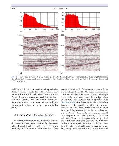
FIG. 6.4 An example stack section (A) before, and (B) after deconvolution and its corresponding mean amplitude spectra
(top). Deconvolution removes the ringy character of the reflections, which is especially evident for the strong reflections at
1300 and 1750 ms.

well-known deconvolution method is predictive synthetic sections. Reflections are acquired from
deconvolution, which tries to estimate and the interfaces defined by the acoustic impedance
remove the multiple reflections from the data. contrasts of the subsurface layers. Although
Among these numerous deconvolution methods the acoustic impedance equals the multiplication
available, spiking and predictive deconvolu- of velocity and density for a specific layer
tions are the most common techniques and have (Section 1.3.2), the densities of the subsurface
widespread applications in the seismic industry layers are not generally considered in acoustic
today. impedance calculations in the case where there
is no well log information in the area, because
the variations of the density values are quite small
6.1 CONVOLUTIONAL MODEL with respect to the velocity changes across the
interfaces. Therefore, it is generally thought that
In order to comprehend the theoretical basis of the subsurface interfaces separate the mediums
deconvolution, one must consider the 1D convo- of different wave velocities, and a reflection coef-
lutional model which underlies 1D seismic ficient can be calculated for each individual inter-
modeling and is used to compute zero-offset face using only the velocities of the media it