Page 369 - Acquisition and Processing of Marine Seismic Data

360 6. DECONVOLUTION

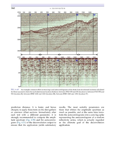
FIG. 6.45 An example common offset section (top) and autocorrelograms of the shots from its selected locations calculated
for three successive shots for each determined location (bottom): between FFID 250 and 252 (location I), between FFID 550 and
552 (location II), between FFID 1030 and 1032 (location III), between FFID 1300 and 1302 (location IV).

prediction distance. It is faster, and hence results. The most suitable parameters are
cheaper, to apply these tests on the shot gathers those that whiten the amplitude spectrum as
or common offset sections. Immediately after much as possible, and at the same time trans-
each test with a different parameter, it is form the autocorrelograms into a zero lag spike
strongly recommended to compute the ampli- representing the autocorrelogram of a random
tude spectrum (Fig. 6.50) and the autocorrelo- reflectivity series, which is actually regarded
gram (Fig. 6.51) of the deconvolution output to as the ultimate goal of the deconvolution
ensure that the application yields satisfactory application.