Page 365 - Acquisition and Processing of Marine Seismic Data

356 6. DECONVOLUTION

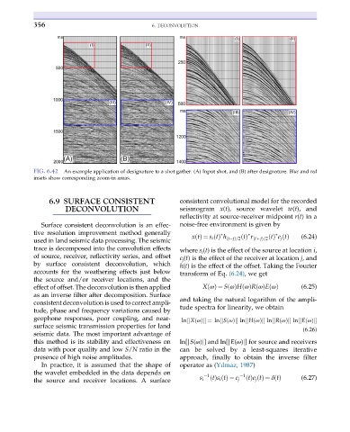
FIG. 6.42 An example application of designature to a shot gather. (A) Input shot, and (B) after designature. Blue and red
insets show corresponding zoom-in areas.

6.9 SURFACE CONSISTENT consistent convolutional model for the recorded
DECONVOLUTION seismogram x(t), source wavelet w(t), and
reflectivity at source-receiver midpoint r(t)in a
Surface consistent deconvolution is an effec- noise-free environment is given by
tive resolution improvement method generally ∗ ∗ ∗ (6.24)
ð
used in land seismic data processing. The seismic xtðÞ ¼ s i tðÞ h i jð Þ=2 tðÞ r i + jÞ=2 tðÞ e j tðÞ
trace is decomposed into the convolution effects where s i (t) is the effect of the source at location i,
of source, receiver, reflectivity series, and offset e j (t) is the effect of the receiver at location j, and
by surface consistent deconvolution, which h(t) is the effect of the offset. Taking the Fourier
accounts for the weathering effects just below transform of Eq. (6.24), we get
the source and/or receiver locations, and the
effect of offset. The deconvolution is then applied X ωðÞ ¼ S ωðÞH ωðÞR ωðÞE ωðÞ (6.25)
as an inverse filter after decomposition. Surface
and taking the natural logarithm of the ampli-
consistent deconvolution is used to correct ampli-
tude spectra for linearity, we obtain
tude, phase and frequency variations caused by
geophone responses, poor coupling, and near-
j ½
j ½
j ½
j ½
j ½
ln X ωðÞjŠ ¼ ln S ωðÞjŠ ln H ωðÞjŠ ln R ωðÞjŠ ln E ωðÞjŠ
surface seismic transmission properties for land
(6.26)
seismic data. The most important advantage of
this method is its stability and effectiveness on ln[jS(ω)j] and ln[jE(ω)j] for source and receivers
data with poor quality and low S/N ratio in the can be solved by a least-squares iterative
presence of high noise amplitudes. approach, finally to obtain the inverse filter
In practice, it is assumed that the shape of operator as (Yılmaz, 1987)
the wavelet embedded in the data depends on
1 1 t (6.27)
the source and receiver locations. A surface s i t ðÞs i tðÞ ¼ e j ðÞe j tðÞ ¼ δ tðÞ