Page 399 - Acquisition and Processing of Marine Seismic Data

390 7. SUPPRESSION OF MULTIPLE REFLECTIONS

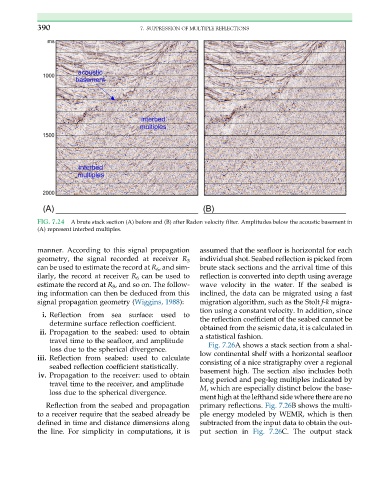
FIG. 7.24 A brute stack section (A) before and (B) after Radon velocity filter. Amplitudes below the acoustic basement in
(A) represent interbed multiples.

manner. According to this signal propagation assumed that the seafloor is horizontal for each
geometry, the signal recorded at receiver R 3 individual shot. Seabed reflection is picked from
can be used to estimate the record at R 6 , and sim- brute stack sections and the arrival time of this
ilarly, the record at receiver R 6 can be used to reflection is converted into depth using average
estimate the record at R 8 , and so on. The follow- wave velocity in the water. If the seabed is
ing information can then be deduced from this inclined, the data can be migrated using a fast
signal propagation geometry (Wiggins, 1988): migration algorithm, such as the Stolt f-k migra-
tion using a constant velocity. In addition, since
i. Reflection from sea surface: used to
the reflection coefficient of the seabed cannot be
determine surface reflection coefficient.
obtained from the seismic data, it is calculated in
ii. Propagation to the seabed: used to obtain
a statistical fashion.
travel time to the seafloor, and amplitude
Fig. 7.26A shows a stack section from a shal-
loss due to the spherical divergence.
low continental shelf with a horizontal seafloor
iii. Reflection from seabed: used to calculate
consisting of a nice stratigraphy over a regional
seabed reflection coefficient statistically.
basement high. The section also includes both
iv. Propagation to the receiver: used to obtain
long period and peg-leg multiples indicated by
travel time to the receiver, and amplitude
M, which are especially distinct below the base-
loss due to the spherical divergence.
ment high at the lefthand side where there are no
Reflection from the seabed and propagation primary reflections. Fig. 7.26B shows the multi-
to a receiver require that the seabed already be ple energy modeled by WEMR, which is then
defined in time and distance dimensions along subtracted from the input data to obtain the out-
the line. For simplicity in computations, it is put section in Fig. 7.26C. The output stack