Page 276 - Adaptive Identification and Control of Uncertain Systems with Nonsmooth Dynamics

278 Adaptive Identification and Control of Uncertain Systems with Non-smooth Dynamics

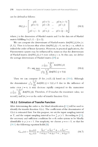
can be defined as follows:
⎡ ⎤
y(l) y(l + 1) ... y(l + j − 1)
⎢ y(l + 1) y(l + 2)... y(l + j) ⎥
⎢
(18.5)
⎥
H(l,j) = ⎢ ⎥
... ... ... ...
⎣ ⎦
y(l + j − 1) y(l + j) ... y(l + 2j − 2)
where j is the dimension of Hankel matrix and l is the data set of Hankel
matrix fulfilling l ∈[1,L − 2j + 2].
We can compute the determinant of Hankel matrix det[H(l,j)] for j ∈
[1,L]. Then it is known that when det[H(l,j)]= 0, we let j = n,which is
indeed the order of linear dynamics. However, in practical applications, the
Hammerstein system may be influenced by noises so that the determinant
of Hankel matrix det[H(l,j)] = 0even when j = n. In this case, we define
the average determinant of Hankel matrix [20]as

L−2j+2
1
L−2j+2 det[H(l,j)]
D = arg max l=1 . (18.6)
1 j L L−2j
1
L−2j det[H(l,(j + 1))]
l=1
Then we can compute D for j ∈[1,L] based on (18.6). Although
L−2j
the denominator 1
det[H(l,(j + 1))] = 0 due to the influence of
L−2j
l=1
noise even j = n, it may decrease rapidly compared to the numerator
L−2j+2
1
L−2j+2 det[H(l,j)]. Therefore, if D reaches the maximum value, we
l=1
record j and let j = n as the order of transfer function G(z).

18.3.2 Estimation of Transfer Function
After determining the order n, the blind identification [11]willbeusedto
identify the transfer function G(z). The coefficients of the denominator of
G(z) is estimated first. For this purpose, we set the input sampling interval
T
as T, and the output sampling interval as h = ,ρ 1. According to [11],
ρ
the necessary and sufficient condition for n-th order system to be blindly
identifiable is ρ n + 1. For simplicity, we choose ρ = n + 1, so that for
(18.1) the following equation holds [8]:

¯
y n+1 (z) b 1z −1 + b 2z −2 + ... + b nz −n
¯
¯
G n+1 (z) = = (18.7)
x n+1 (z) 1 +¯a 1z −1 +¯a 2z −2 + ... +¯a nz −n