Page 297 - Adaptive Identification and Control of Uncertain Systems with Nonsmooth Dynamics

300 Adaptive Identification and Control of Uncertain Systems with Non-smooth Dynamics

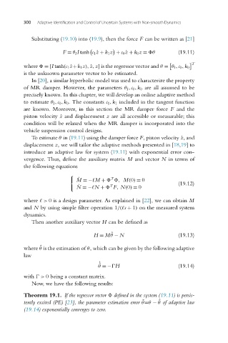
Substituting (19.10)into(19.9), then the force F canbewrittenas[21]

F = θ I I tanh c 1 ˙z + k 1z + c 0 ˙z + k 0z = θ (19.11)
T

where =[I tanh(c 1 ˙z+k 1z), ˙z,z] is the regressor vector and θ = θ I ,c 0 ,k 0
is the unknown parameter vector to be estimated.
In [20], a similar hyperbolic model was used to characterize the property
of MR damper. However, the parameters θ I ,c 0 ,k 0 are all assumed to be
precisely known. In this chapter, we will develop an online adaptive method
to estimate θ I ,c 0 ,k 0. The constants c 1 ,k 1 included in the tangent function
are known. Moreover, in this section the MR damper force F and the
piston velocity ˙z and displacement z are all accessible or measurable; this
condition will be relaxed when the MR damper is incorporated into the
vehicle suspension control designs.
To estimate θ in (19.11) using the damper force F, piston velocity ˙z,and
displacement z, we will tailor the adaptive methods presented in [18,19]to
introduce an adaptive law for system (19.11) with exponential error con-
vergence. Thus, define the auxiliary matrix M and vector N in terms of
the following equations

T
˙ M =− M + , M(0) = 0
(19.12)
T
˙ N =− N + F, N(0) = 0
where > 0 is a design parameter. As explained in [22], we can obtain M
and N by using simple filter operation 1/( s + 1) on the measured system
dynamics.
Then another auxiliary vector H can be defined as

ˆ
H = Mθ − N (19.13)
where θ is the estimation of θ, which can be given by the following adaptive
ˆ
law
˙
θ =− H (19.14)
ˆ
with > 0 being a constant matrix.
Now, we have the following results:
Theorem 19.1. If the regressor vector defined in the system (19.11) is persis-
tently excited (PE) [23], the parameter estimation error θ=θ − θ of adaptive law
˜
ˆ
(19.14) exponentially converges to zero.