Page 299 - Adaptive Identification and Control of Uncertain Systems with Nonsmooth Dynamics
P. 299

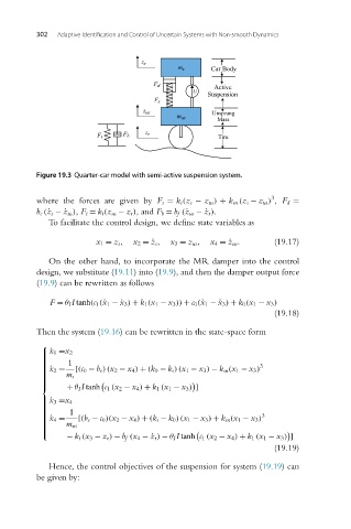
302   Adaptive Identification and Control of Uncertain Systems with Non-smooth Dynamics


                        Figure 19.3 Quarter-car model with semi-active suspension system.

                                                                                  3
                        where the forces are given by F s = k s (z s − z us ) + k sn (z s − z us ) , F d =
                        b e (˙ z s −¨z us ), F t = k t (z us − z r ),and F b = b f (˙ z us −¨z r ).
                           To facilitate the control design, we define state variables as

                                       x 1 = z s ,  x 2 =˙z s ,  x 3 = z us ,  x 4 =˙z us .  (19.17)

                           On the other hand, to incorporate the MR damper into the control
                        design, we substitute (19.11)into(19.9), and then the damper output force
                        (19.9)can be rewrittenasfollows

                            F = θ I I tanh(c 1 (˙x 1 −¨x 3 ) + k 1 (x 1 − x 3 )) + c 0 (˙x 1 −¨x 3 ) + k 0 (x 1 − x 3 )
                                                                                   (19.18)

                        Then the system (19.16) can be rewritten in the state-space form

                          ⎧
                          ⎪ ˙ x 1 =x 2
                          ⎪
                                1
                          ⎪
                          ⎪
                          ⎪
                          ⎪                                                    3
                          ⎪ ˙x 2 =  [(c 0 − b e )(x 2 − x 4 ) + (k 0 − k s )(x 1 − x 3 ) − k sn (x 1 − x 3 )
                          ⎪
                                m s
                          ⎪
                          ⎪
                          ⎪
                          ⎪

                          ⎪
                                + θ I I tanh c 1 (x 2 − x 4 ) + k 1 (x 1 − x 3 ) ]
                          ⎨
                          ⎪ ˙ x 3 =x 4
                          ⎪
                          ⎪
                                1
                          ⎪
                          ⎪
                          ⎪                                                     3
                          ⎪
                          ⎪ ˙x 4 =  [(b e − c 0 )(x 2 − x 4 ) + (k s − k 0 )(x 1 − x 3 ) + k sn (x 1 − x 3 )
                          ⎪
                                m us
                          ⎪
                          ⎪
                          ⎪
                          ⎪

                          ⎩
                                − k t (x 3 − z r ) − b f (x 4 −¨z r ) − θ I I tanh c 1 (x 2 − x 4 ) + k 1 (x 1 − x 3 ) ]
                                                                                   (19.19)
                           Hence, the control objectives of the suspension for system (19.19)can
                        be given by:
   294   295   296   297   298   299   300   301   302   303   304