Page 303 - Adaptive Identification and Control of Uncertain Systems with Nonsmooth Dynamics
P. 303

306   Adaptive Identification and Control of Uncertain Systems with Non-smooth Dynamics


                        19.3.3 Suspension Performance Analysis
                        The convergence of x 1 has been guaranteed based on Theorem 19.2.In
                        the following, we will address the other two suspension performance re-
                        quirements (19.20)and (19.21).
                           First, the boundedness of the state variables x 3 ,x 4 of system (19.19)
                        is studied. Substituting (19.26)into(19.19), one can obtain the following
                        dynamics

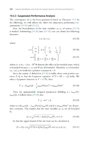
                                                    ˙ x = Ax + ω                   (19.35)
                        where


                                                             0     1
                                                x 3
                                          x =       ,A =                           (19.36)
                                                             k t   b f
                                                x 4        −     −
                                                             m us  m us

                                                          0
                                            ω =                                    (19.37)
                                                  k t    b f   m s
                                                    z r +  ˙ z r +  ω 1
                                                  m us  m us   m us
                                              ˜ T
                        where ω 1 = k ss 1 + x 2 −
   denotes the effect of the residual error, which
                        is bounded because s 1 ,x 2 and 
 are all bounded. Therefore, ω is bounded,
                                                   ˜
                        i.e.,  ω  ≤   holds for a positive constant  > 0.
                           Since the matrix A defined in (19.36) is stable, there exist positive ma-
                                                                 T
                        trices P,Q so that the Lyapunov equation A P + AP =−Q holds. We
                                                        T
                        select a Lyapunov function as V = x Px,then
                                                 1
                                                             2
                                  ˙ V ≤−[λ min (Q) − λ max (P)] x  + ηλ max (P)  2  (19.38)
                                                 η
                           Then for appropriately designed parameters fulfilling η> λ max (P)/
                        λ min (Q), it follows from (19.38)that
                                                   ˙ V ≤−αV + β                    (19.39)

                                                                              2
                        where α =[λ min (Q) − λ max (P)/η]/λ min (P) and β = ηλ max (P)  are all pos-
                        itive constants. This implies that the state variables x 3 ,x 4 are all bounded
                        by


                                        |x i | ≤  (V(0) + β α) λ min (P),i = 3,4   (19.40)
                           So that the upper bound of the tire load can be calculated as


                              |F t + F b | ≤ k t (V(0) + β α) λ min (P) + k t |z r | + b f |˙ z r |  (19.41)
   298   299   300   301   302   303   304   305   306   307   308