Page 58 - Adaptive Identification and Control of Uncertain Systems with Nonsmooth Dynamics

Adaptive Dynamic Surface Control of Two-Inertia Systems With LuGre Friction Model 49

3.3.4 Stability Analysis
In this section, the stability of the closed-loop system is proved by using
Lyapunov stability theory. The main results can be summarized in the fol-
lowing theorem.

Theorem 3.1. Consider the two-inertia system (3.1), the controller (3.49)with
(3.29), (3.35), and friction compensation (3.48), adaptive laws (3.45)and (3.47)
are used, then all signals in the closed-loop system are semi-globally uniformly ulti-
mately bounded (SGUUB). Moreover, the tracking error s 1 can be guaranteed within
the bound specified by the selected PPF μ 1 (t).
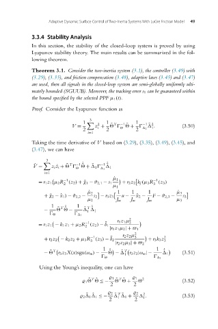
Proof. Consider the Lyapunov function as

3
1 2 1 T −1 1 −1 2
˜
˜
˜
V = z + + . (3.50)

1
i
2 2 2 1
i=1
Taking the time derivative of V based on (3.29), (3.35), (3.49), (3.45), and
(3.47), we can have
3
T −1 ˙ −1 ˙
˙ V = z ˜ ˜ ˜ ˜
z i ˙ i + + 1 1
1
i=1
−1 −1
˙ μ 1
= r 1z 1 μ 2R (z 2 ) +¯χ 1 − ϑ 2,1 − s 1 + r 2z 2 k f (μ 3R (z 3 )
2 3
μ 1
1 1 1
˙ μ 2 ˙ μ 3
+¯χ 2 − x 1 ) − ϑ 2,2 − s 2 − r 3z 3 u − ˆ x 2 − F − ϑ 2,3 − s 3
μ 2 J m J m J m μ 3
1 1
T ˙
T ˙
ˆ
˜
ˆ
˜
− − 1
1
1
r 1z 1 μ 2
−1 ¯ 2

= r 1z 1 − k 1z 1 + μ 2R (z 2 ) − δ 1
2
|r 1z 1 μ 2 |+ 1
r 2z 2 μ 2
−1 3 2

¯
+ r 2z 2 − k 2z 2 + μ 3R (z 3 ) − δ 2 + r 3k 3z 3
3
|r 2z 2 μ 3 |+ 2
1 1

˜ T ˙ ˆ ˜ T ˙ ˆ
− r 3z 3X(x)sgn(ω m ) − − r 3z 3 |ω m |− 1 (3.51)
1
1
Using the Young’s inequality, one can have
T
T
˜
˜
ˆ
˜
1 ≤− 1 + 1 2 (3.52)
2 2
2 T 2 2
˜ ˆ
˜
˜
2 1 1 ≤− 1 + . (3.53)
1
1
2 2