Page 613 - Advanced_Engineering_Mathematics o'neil

16.5 Laplace Transform Techniques 593

2

h(t)
1

(0,1)
0
0 0.2 0.4 0.6 0.8 1
x t
(4L/c, 0) (8L/c, 0)
–1

–2

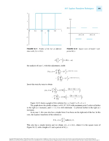
FIGURE 16.11 Profiles of the bar at different FIGURE 16.12 Square wave of height 1 and
times with f (t) = Iδ(t). period 4L/c.

1
L e −αs = H(t − α)
s
the analysis of case 1, with this adjustment, yields
∞
cI
1
Y(x,s) = (−1) n e −(((2n+1)L−x)/c)s
E s
n=0
∞
cI
1
− (−1) n e −(((2n+1)L+x)/c)s .
E s
n=0
Invert this term by term to obtain
∞
cI
n (2n + 1)L − x
y(x,t) = (−1) H t −
E c
n=0
∞
cI
n (2n + 1)L + x
− (−1) H t − .
E c
n=0
Figure 16.11 shows a graph of this solution for c = 2 and I = E = L = 1.
The graph shows the profile at times t =0.4,0.7,0.9 (with maximum point 2 achieved farther
to the right as t increases, and t = 1.3,1.8, with minimum −2 achieved farther to the right as t
increases.
As in case 1, this case also has a simple form if we focus on the right end of the bar. In this
case, the Laplace transform of the solution is

cI 1
Y(L,s) = tanh(sL/c).
E s
This also has a simple inverse and we obtain y(L,s) = h(t), where h is the square wave of
Figure 16.12, with a height of 1 and a period of 4L/c.

Copyright 2010 Cengage Learning. All Rights Reserved. May not be copied, scanned, or duplicated, in whole or in part. Due to electronic rights, some third party content may be suppressed from the eBook and/or eChapter(s).
Editorial review has deemed that any suppressed content does not materially affect the overall learning experience. Cengage Learning reserves the right to remove additional content at any time if subsequent rights restrictions require it.

October 14, 2010 15:23 THM/NEIL Page-593 27410_16_ch16_p563-610