Page 124 - Advanced engineering mathematics

104 CHAPTER 3 The Laplace Transform

EXAMPLE 3.17
We will solve

y + 2y + 2y = δ(t − 3); y(0) = y (0) = 0.

Apply the transform to the differential equation to get
2
s Y(s) + 2sY(s) + 2Y(s) = e −3s ,

so
1
Y(s) = e −3s .
2
s + 2s + 2
The solution is the inverse transform of Y(s). To compute this, first write

1 −3s
Y(s) = e .
(s + 1) + 1
2
−1
2
Because L [1/(s + 1)]= sin(t),ashiftinthe s− variable gives us

1
−1 −t
L = e sin(t).
(s + 1) + 1
2
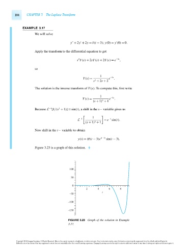
Now shift in the t− variable to obtain
y(t) = H(t − 3)e (t−3) sin(t − 3).

Figure 3.23 is a graph of this solution.

100

50

0
2 4 6 8
t
–50
–100

–150

FIGURE 3.23 Graph of the solution in Example
3.17.

Copyright 2010 Cengage Learning. All Rights Reserved. May not be copied, scanned, or duplicated, in whole or in part. Due to electronic rights, some third party content may be suppressed from the eBook and/or eChapter(s).
Editorial review has deemed that any suppressed content does not materially affect the overall learning experience. Cengage Learning reserves the right to remove additional content at any time if subsequent rights restrictions require it.

October 14, 2010 14:14 THM/NEIL Page-104 27410_03_ch03_p77-120