Page 158 - Advanced engineering mathematics

138 CHAPTER 5 Approximation of Solutions

2

1

–2 –1 y(x)=0 1 2

–1

–2
2

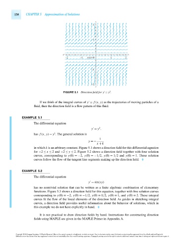
FIGURE 5.1 Directionfieldfor y = y .
If we think of the integral curves of y = f (x, y) as the trajectories of moving particles of a

fluid, then the direction field is a flow pattern of this fluid.

EXAMPLE 5.1
The differential equation
2

y = y .
2
has f (x, y) = y . The general solution is
1
y =−
x + k
in which k is an arbitrary constant. Figure 5.1 shows a direction field for this differential equation
for −2 ≤ x ≤ 2 and −2 ≤ y ≤ 2. Figure 5.2 shows a direction field together with four solution
curves, corresponding to y(0) =−2, y(0) =−1/2, y(0) = 1/2 and y(0) = 1. These solution
curves follow the flow of the tangent line segments making up the direction field.

EXAMPLE 5.2
The differential equation

y = sin(xy)
has no nontrivial solution that can be written as a finite algebraic combination of elementary
functions. Figure 5.3 shows a direction field for this equation, together with five solution curves
corresponding to y(0) =−2, y(0) =−1/2, y(0) = 1/2, y(0) = 1, and y(0) = 2. These integral
curves fit the flow of the lineal elements of the direction field. As guides in sketching integral
curves, a direction field provides useful information about the behavior of solutions, which in
this example we do not have explicitly in hand.

It is not practical to draw direction fields by hand. Instructions for constructing direction
fields using MAPLE are given in the MAPLE Primer in Appendix A.

Copyright 2010 Cengage Learning. All Rights Reserved. May not be copied, scanned, or duplicated, in whole or in part. Due to electronic rights, some third party content may be suppressed from the eBook and/or eChapter(s).
Editorial review has deemed that any suppressed content does not materially affect the overall learning experience. Cengage Learning reserves the right to remove additional content at any time if subsequent rights restrictions require it.

October 14, 2010 14:19 THM/NEIL Page-138 27410_05_ch05_p137-144