Page 163 - Advanced engineering mathematics

5.3 Taylor and Modified Euler Methods 143

EXAMPLE 5.4

We will use the second-order Taylor method to approximate some solution values for y =
2
y cos(x); y(0)=1/5. This problem can be solved exactly to obtain y(x)=1/(5−sin(x)),sowe
can compare approximate values with exact values.
2
2
With f (x, y) = y cos(x), f x =−y sin(x) and f y = 2y cos(x). The second-order Taylor
approximation formula is
1
2
2
2
2
2
2
y k+1 = y k + hy cos(x k ) + h y cos (x k ) − h y sin(x k ).
k k k
2
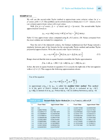
Table 5.2 lists approximate values computed using h = 0.2 and n = 20. Values computed from
the exact solution are included for comparison.
Near the end of the nineteenth century, the German mathematician Karl Runge noticed a
similarity between part of the formula for the second-order Taylor method and another Taylor
polynomial approximation. Write this second-order Taylor formula as
1

y k+1 = y k + h f k + h( f x (x k , y k ) + f k f y (x k , y k )) . (5.2)
2
Runge observed that the term in square brackets resembles the Taylor approximation
f (x k + αh, y k + βh)) ≈ f k + αhf x (x k , y k ) + βhf y (x k , y k ).
In fact, the term in square brackets in equation (5.2) is exactly the right side of the last equation
with α = β = 1/2. This suggests the following approximation scheme.

Use of the equation
h hf k

y k+1 ≈ y k + hf x k + , y k + .
2 2
to approximate y(x k+1 ) by y k+1 is called the modified Euler method. This method
is in the spirit of Euler’s method except that f (x, y) is evaluated at (x k + h/2,
y k + hf k /2) instead of at (x k , y k ). Notice that x k + h/2 is midway between x k and x k + h.

2

TABLE 5.2 Second-Order Taylor Method for y = y cos(x); y(0) = 1/5
x Exact Value Approximate Value x Exact Value Approximate Value

0.0 0.2 0.2 2.2 0.2385778700 0.2389919589
0.2 0.2082755946 0.20832 2.4 0.2312386371 0.2315347821
0.4 0.2168923737 0.2170013470 2.6 0.2229903681 0.2231744449
0.6 0.2254609677 0.2256558280 2.8 0.2143617277 0.2144516213
0.8 0.2335006181 0.2337991830 3.0 0.2058087464 0.2058272673
1.0 0.2404696460 0.2408797598 3.2 0.197691800 0.1976613648
1.2 0.2458234042 0.2463364693 3.4 0.1902753647 0.1902141527
1.4 0.2490939041 0.2496815188 3.6 0.1837384003 0.1836603456
1.6 0.2499733530 0.2505900093 3.8 0.1781941060 0.1781084317
1.8 0.2483760942 0.2489684556 4.0 0.1737075401 0.1736197077
2.0 0.2444567851 0.2449763987

Copyright 2010 Cengage Learning. All Rights Reserved. May not be copied, scanned, or duplicated, in whole or in part. Due to electronic rights, some third party content may be suppressed from the eBook and/or eChapter(s).
Editorial review has deemed that any suppressed content does not materially affect the overall learning experience. Cengage Learning reserves the right to remove additional content at any time if subsequent rights restrictions require it.

October 14, 2010 14:19 THM/NEIL Page-143 27410_05_ch05_p137-144