Page 160 - Advanced engineering mathematics

140 CHAPTER 5 Approximation of Solutions

, y )
Slope f(x 0 0
y

(x , y )
2
2
, y )
(x 1 1
, y )
(x 3 3
Slope
f(x , y ) (x , y )
0
0
1
1
Slope f(x , y )
2
2
x
x 1 x
x 0 2 x 3
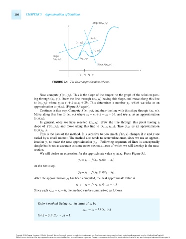
FIGURE 5.4 The Euler approximation scheme.
Now compute f (x 1 , y 1 ). This is the slope of the tangent to the graph of the solution pass-
ing through (x 1 , y 1 ). Draw the line through (x 1 , y 1 ) having this slope, and move along this line
to (x 2 , y 2 ) where y 2 = x 1 + h = x 0 + 2h. This determines a number y 2 , which we take as an
approximation to y(x 2 ). (Figure 5.4 again).
Continue in this way. Compute f (x 2 , y 2 ), and draw the line with this slope through (x 2 , y 2 ).
Move along this line to (x 3 , y 3 ) where x 3 = x 2 + h = x 0 + 3h, and use y 3 as an approximation
to y(x 3 ).
In general, once we have reached (x k , y k ), draw the line through this point having a
slope of f (x k , y k ), and move along this line to (x k+1 , y k+1 ).Take y k+1 as an approximation
to y(x k+1 ).
This is the idea of the method. It is sensitive to how much f (x, y) changes if x and y are
varied by a small amount. The method also tends to accumulate error, since we use an approx-
imation y k to make the next approximation y k+1 . Following segments of lines is conceptually
simple but is not as accurate as some other methods—two of which we will develop in the next
section.
We will derive an expression for the approximate value y k at x k . From Figure 5.4,
y 1 = y 0 + f (x 0 , y 0 )(x 1 − x 0 ).
At the next step,

y 2 = y 1 + f (x 1 , y 1 )(x 2 − x 1 ).
After the approximation y k has been computed, the next approximate value is
y k+1 = y k + f (x k , y k )(x k+1 − x k ).

Since each x k+1 − x k = h, the method can be summarized as follows.

Euler’s method Define y k+1 in terms of y k by
y k+1 = y k + hf (x k , y k )
for k = 0,1,2,··· ,n − 1.

Copyright 2010 Cengage Learning. All Rights Reserved. May not be copied, scanned, or duplicated, in whole or in part. Due to electronic rights, some third party content may be suppressed from the eBook and/or eChapter(s).
Editorial review has deemed that any suppressed content does not materially affect the overall learning experience. Cengage Learning reserves the right to remove additional content at any time if subsequent rights restrictions require it.

October 14, 2010 14:19 THM/NEIL Page-140 27410_05_ch05_p137-144