Page 161 - Advanced engineering mathematics

5.2 Euler’s Method 141

√
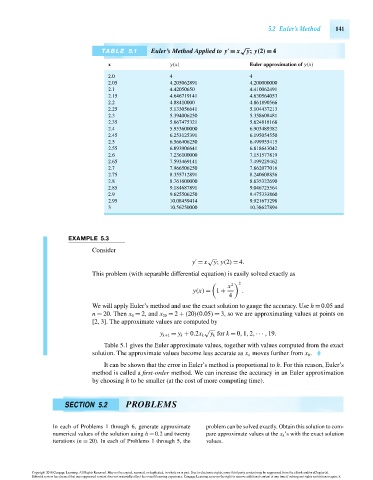
TABLE 5.1 Euler’s Method Applied to y = x y; y(2) = 4

x y(x) Euler approximation of y(x)
2.0 4 4
2.05 4.205062891 4.200000000
2.1 4.42050650 4.410062491
2.15 4.646719141 4.630564053
2.2 4.88410000 4.861890566
2.25 5.133056641 5.104437213
2.3 5.394006250 5.358608481
2.35 5.667475321 5.624818168
2.4 5.953600000 6.903489382
2.45 6.253125391 6.195054550
2.5 6.566406250 6.499955415
2.55 6.893906641 6.818643042
2.6 7.236100000 7.151577819
2.65 7.593469141 7.499229462
2.7 7.966506250 7.862077016
2.75 8.355712891 8.240608856
2.8 8.761600000 8.635322690
2.85 9.184687891 9.046725564
2.9 9.625506250 9.475333860
2.95 10.08459414 9.921673298
3 10.56250000 10.38627894

EXAMPLE 5.3

Consider
√
y = x y; y(2) = 4.

This problem (with separable differential equation) is easily solved exactly as
2
x
2
y(x) = 1 + .
4
We will apply Euler’s method and use the exact solution to gauge the accuracy. Use h =0.05 and
n = 20. Then x 0 = 2, and x 20 = 2 + (20)(0.05) = 3, so we are approximating values at points on
[2,3]. The approximate values are computed by
√
y k+1 = y k + 0.2x k y k for k = 0,1,2,··· ,19.
Table 5.1 gives the Euler approximate values, together with values computed from the exact
solution. The approximate values become less accurate as x k moves further from x 0 .
It can be shown that the error in Euler’s method is proportional to h. For this reason, Euler’s
method is called a first-order method. We can increase the accuracy in an Euler approximation
by choosing h to be smaller (at the cost of more computing time).

SECTION 5.2 PROBLEMS

In each of Problems 1 through 6, generate approximate problem can be solved exactly. Obtain this solution to com-
numerical values of the solution using h = 0.2 and twenty pare approximate values at the x k ’s with the exact solution
iterations (n = 20). In each of Problems 1 through 5, the values.

Copyright 2010 Cengage Learning. All Rights Reserved. May not be copied, scanned, or duplicated, in whole or in part. Due to electronic rights, some third party content may be suppressed from the eBook and/or eChapter(s).
Editorial review has deemed that any suppressed content does not materially affect the overall learning experience. Cengage Learning reserves the right to remove additional content at any time if subsequent rights restrictions require it.

October 14, 2010 14:19 THM/NEIL Page-141 27410_05_ch05_p137-144