Page 164 - Advanced engineering mathematics

144 CHAPTER 5 Approximation of Solutions

2
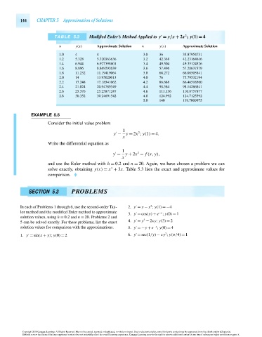
TABLE 5.3 Modified Euler’s Method Applied to y = y/x + 2x ; y(1) = 4

x y(x) Approximate Solution x y(x) Approximate Solution
1.0 4 4 3.0 36 35.87954731
1.2 5.328 5.320363636 3.2 42.368 42.23164616
1.4 6.944 6.927398601 3.4 49.504 49.35124526
1.6 8.896 8.869292639 3.6 57.496 57.28637379
1.8 11.232 11.19419064 3.8 66.272 66.08505841
2.0 14 13.95020013 4.0 76 75.79532194
2.2 17.248 17.18541062 4.2 86.688 86.46518560
2.4 21.024 20.94789549 4.4 98.384 98.14266841
2.6 25.376 25.25871247 4.6 111.136 110.8757877
2.8 30.352 30.24691542 4.8 124.992 124.7125592
5.0 140 139.7009975

EXAMPLE 5.5
Consider the initial value problem
1
2
y − y = 2x ; y(1) = 4.
x
Write the differential equation as
1
2
y = y + 2x = f (x, y),
x
and use the Euler method with h = 0.2 and n = 20. Again, we have chosen a problem we can
3
solve exactly, obtaining y(x) = x + 3x. Table 5.3 lists the exact and approximate values for
comparison.

SECTION 5.3 PROBLEMS

2
In each of Problems 1 through 6, use the second-order Tay- 2. y = y − x ; y(1) =−4

lor method and the modified Euler method to approximate −x
3. y = cos(y) + e ; y(0) = 1

solution values, using h = 0.2and n = 20. Problems 2 and
3

5 can be solved exactly. For these problems, list the exact 4. y = y − 2xy; y(3) = 2
−x
solution values for comparison with the approximations. 5. y =−y + e ; y(0) = 4

2

1. y = sin(x + y); y(0) = 2 6. y = sec(1/y) − xy ; y(π/4) = 1

Copyright 2010 Cengage Learning. All Rights Reserved. May not be copied, scanned, or duplicated, in whole or in part. Due to electronic rights, some third party content may be suppressed from the eBook and/or eChapter(s).
Editorial review has deemed that any suppressed content does not materially affect the overall learning experience. Cengage Learning reserves the right to remove additional content at any time if subsequent rights restrictions require it.

October 14, 2010 14:19 THM/NEIL Page-144 27410_05_ch05_p137-144