Page 98 - Advanced engineering mathematics

78 CHAPTER 3 The Laplace Transform

and so on. If we include the variable, these would be written
L[ f ](s) = F(s), L[g](s) = G(s), and L[h](s) = H(s)
It is also customary to use t (for time) as the variable of the input function and s for the variable
of the transformed function.

EXAMPLE 3.1
at
Let a be any real number, and f (t) = e . The Laplace transform of f is the function defined by
∞

e dt
L[ f ](s) = e −st at
0
∞
k
= e (a−s)t dt = lim e (a−s)t dt
k→∞
0 0
k
1

= lim e (a−s)t
k→∞ a − s
0
1 1
=− =
a − s s − a
at
provided that s > a. The Laplace transform of f (t) = e can be denoted F(s) = 1/(s − a) for
s > a.
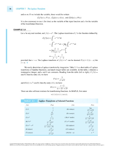
We rarely determine a Laplace transform by integration. Table 3.1 is a short table of Laplace
transforms of familiar functions, and much longer tables are available. In this table, n denotes a
nonnegative integer, and a and b are constants. Reading from the table (left to right), if f (t) =
sin(3t) then by entry (6), we have
3
F(s) = ,
2
s + 9
2t
and if k(t) = e cos(5t) then by entry (11), we have
s − 2
K(s) = .
(s − 2) + 25
2
There are also software routines for transforming functions. In MAPLE, first enter
with(inttrans);

TABLE 3.1 Laplace Transforms of Selected Functions

f (t) F(s) f (t) F(s)
1 2as
(1) 1 (8) t sin(at)
2
s (s + a )
2 2
2
n! s − a 2
(2) t n (9) t cos(at)
2 2
2
s n+1 (s + a )
1 b
at
(3) e at (10) e sin(bt)
s − a (s − a) + b 2
2
n! s − a
n at
(4) t e (11) e cos(bt)
at
(s − a) n+1 (s − a) + b 2
2
a − b a
at
(5) e − e bt (12) sinh(at)
(s − a)(s − b) s − a 2
2
a s
(6) sin(at) (13) cosh(at)
s + a 2 s − a 2
2
2
s
(7) cos(at) (14) δ(t − a) e −as
s + a 2
2
Copyright 2010 Cengage Learning. All Rights Reserved. May not be copied, scanned, or duplicated, in whole or in part. Due to electronic rights, some third party content may be suppressed from the eBook and/or eChapter(s).
Editorial review has deemed that any suppressed content does not materially affect the overall learning experience. Cengage Learning reserves the right to remove additional content at any time if subsequent rights restrictions require it.
October 14, 2010 14:14 THM/NEIL Page-78 27410_03_ch03_p77-120